This module will provide an introduction to methods for analyzing
text. Text analytics is a complicated topic, covering a wide range of
problems and solutions. For example, consider the following simple
questions. How should text data be structured? What types of analysis
are appropriate for text data? How can these analyses be performed? How
should results from text analytics be presented to a viewer?
We will focus on simple approaches to address each of these
questions. In particular, we will discuss different ways to represent
text, and present the use of term frequency to structure a document's
text. We will then present algorithms that use this approach to
measure the similarity between text, to cluster text into topics, to
estimate the sentiment in text, and to present text and text analytics
results to a viewer.
Why Text Analytics?
Much of the data now being captured and stored
is semi-structured or unstructured: it is not being
saved in a structured format, for example, in a database or data
repository with a formal framework. Text data often makes up a large
part of these unstructured collections: email, web pages, news
articles, books, social network postings, and so on. Text analytics
and text mining are meant to be applied to this type of data to
"...find interesting regularities in large textual datasets..." (Fayad)
"...find semantic and abstract information from the surface form of textual data..." (Grobelnik & Mladenic)
where interesting means non-trivial, hidden, previously unknown,
and potentially useful.
Text analytics has many potential applications. These can be
discovery driven, where we try to answer specific questions
through text mining, or data driven, where we take a large
collection of text data and try to derive useful information by
analyzing it.
There are many reasons why analyzing text is difficult.
Abstract. The concepts contained in text are often
difficult to identify and represent (e.g., sentiment or
sarcasm, "I loved the way you put that. No, really, I LOVED it.")
Relationships. Subtle, complex relationships between
concepts must be extracted (e.g., negation, "I thought I'd
enjoy that movie, but in the end it just didn't work out the way I
expected.")
Scale. A document can contain many thousands of words, and
a document collection can contain thousands or hundreds of thousands
of documents.
Each homework group will complete a text analytics assignment. This
involves choosing a problem of interest to address, identifying and
collecting appropriate text data to support the problem, then using
text analysis techniques discussed during this module to analyze your
data and form conclusions and results that will be presented in class.
Sept. 27, 11:59pm
Submit a draft proposal via the Moodle section on Text Mining (Text
Mining Project Proposal Submission) that describes the problem you
will investigate. As taught in communications, the proposal must be
a Word document so we can return comments through change
tracking. The proposal must include the following items.
A problem statement explaining the issue you want to study and
the goals you plan to achieve.
A description of the dataset(s) you will use, detailing either
where the data is available, or how it will be collected. Provide
enough specificity for us to confirm that the data will be
available in a timely manner.
A description of the types of analysis you plan to apply to
your datasets to achieve the goals listed in your problem
statement.
A detailed justification of why the data you plan to
collect will support the problem and analysis you propose to
complete. Projects that we do not feel have a high probability of
success will be returned and will need to be improved or replaced
with a different proposal.
A list of the results you will present at the end of your
analysis.
The draft proposal should be approximately one page in length. We
have provided an
example draft proposal to give you an idea of its length,
content, and format.
Oct. 2, 11:59pm
Submit a revised proposal through the Moodle section on Text Mining
(Text Mining Project Revised Submission) that addresses comments
and/or concerns made by the instructors on your draft proposal. The
revised proposal represents a template for what we expect to see
during your final presentation.
Present your project and its results to the class. Each group will
be allotted 10 minutes: 8 minutes to present, and 2 minutes to
answer one or two questions. Because of our tight schedule, each
group must provide their slides to Andrea by 5pm on Oct. 16 through
the Moodle section on Text Mining (Text Mining Project
Submission). This will allow us to review the presentations
ahead of time. During presentations, groups will screen share their
slides, so you are expected to be prepared and ready to being
presenting immediately when your group is scheduled. Each group
will be strictly limited to 10 minutes for their presentations
(i.e., 4–5 slides for the average presentation). Please
plan your presentations accordingly. For example, consider having
only 1 or 2 groups members present your slides, then have the entire
team available for questions at the end.
You must attend all of the presentations for your cohort. Attending
presentations for the opposite cohort is optional, but certainly
encouraged if you want to see the work they did.
NLTK, Gensim, and Scikit-Learn
Throughout this module we will provide code examples in Python using
the Natural Language
Toolkit (NLTK). NLTK is designed to support natural language
processing and analysis of human language data. It includes the
ability to perform many different language processing operations,
including all of the text analytics techniques we will be discussing.
For techniques beyond the scope of NLTK, we will provide Python
examples that use Gensim, a more sophisticated text analysis package
that includes the text similarity algorithms we will discuss during
the module. We will also discuss the text analytics preprocessing
capabilities built into scikit-learn, and the full NLP package
spaCy.
spaCy
Since spaCy is a much more complicated Python package, we will offer
a brief overview here. spaCy implements a convolution neural net
(CNN)-trained set of statistical models and processing pipelines to
support common natural language processing (NLP) tasks including
tokenization, part-of-speech tagging, named entity recognition,
lemmatization, and support for many different languages. spaCy is
kept up-to-date through regular updates and improvements to its code
base.
Don't worry if terms like "part-of-speech tagging" or
"lemmatization" are unfamiliar. All of these will be covered in
detail during this module, including code examples in both spaCy and
other Python packages.
In order to install spaCy in your Anacoda environment, executed
the Anacode Prompt and enter the following at the
command line.
conda install -c conda-forge spacy
Although the above command installs the spaCy package into your
Anaconda environment, spaCy's strength comes from a set of pre-trained
CNN models. Each model is pre-loaded manually from the Anaconda
Prompt to make it available to spaCy. These are the pre-trained
English language models spaCy provides, along with a brief description
of what their makeup and intended purpose is.
English text pipeline optimized for GPU DNN processing. Includes
transformer,
tagger,
parser,
ner,
attribute_ruler,
lemmatizer.
In order to pre-load a spaCy trained model into your Anaconda
environment, execute the following command from the Anaconda
Prompt with the name of the library provided. For example, to
pre-load
the en_core_web_sm, en_core_web_md,
and en_core_web_lg models, you would execute the
following command. Note, spacy must already be installed
for these commands to work.
Once the required model is downloaded, it can be loaded with
spaCy's load() command.
% import spacy
%
% nlp = spacy.load( 'en_core_web_sm' )
% doc = nlp( "This is a sentence." )
Alternatively, you can import a spaCy model directly in
your Python code. The model still needs to be downloaded before it
can be imported.
% import spacy
% import en_core_web_md
%
% nlp = en_core_web_md.load()
% doc = nlp( "This is a sentence." )
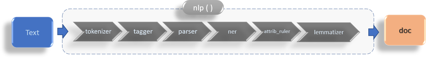
In both cases, spaCy uses its NLP pipeline to convert the text you
provide into a wide range of text properties. The standard pipeline
runs in the following fashion.
tokenizer: converts text into words and punctuation
tokens,
tagger: performs part-of-speech tagging,
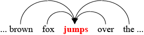
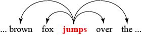
parser: performs dependency parsing to find the structure
and relationships between words in a sentence,
NER: performs named entity recognition,
attribute ruler: performs any user-assigned rules
(e.g.word/phrase token matching), and
lemmatizer: performs lemmatization to convert terms to a
common base form.
All of the various properties spaCy identifies are available in the
doc object. For example, the following simple code
snippet performs NER and returns the entities and the spaCy
estimation of what they represent.
% import spacy
%
% nlp = spacy.load( 'en_core_web_md' )
%
% txt = 'On October 23, Apple CEO Tim Cook Unveiled the new iPad Mini, fourth generation iPad with Retina display, new iMac, and the 13-inch MacBook Pro with Retina display.'
%
% doc = nlp( txt )
%
% for NE in doc.ents:
% print( NE.text, ': ', NE.label_ )
%
October 23 : DATE
Apple : ORG
Tim Cook : PERSON
iPad Mini : PERSON
fourth : ORDINAL
iPad : ORG
Retina : ORG
iMac : ORG
13-inch : QUANTITY
You can view spaCy as a high-level NLP engine, capable of completing
all of the preprocessing steps in preparation for follow-on analysis
in a single nlp() call. Preprocessing is performed
based in large part on the pre-trained models spaCy
encapsulates. The advantage, of course, is that this significantly
reduces the effort needed to get to an analysis point in your
programming. The potential disadvantage is that, although spaCy
allows control of the steps it performs, these may not provide the
fine-grained control needed, and even when it does, it may be just
as much work to tune spaCy versus performing the individual steps
manually. Still, spaCy is a high quality and commonly used option in
the text analytics area.
Text Representations
There are many different ways to represent text. We describe some of
the most common approaches, discussing briefly their advantages and
disadvantages.
Character
The simplest representation views text as an ordered collection of
characters. A text document is described by the frequency of sequences
of characters of different lengths. For example, consider the
following text data.
To be or not to be
This could be represented by a set of single character frequencies
fq (1-grams), a set of two-character frequencies (2-grams), and
so on.
b
e
n
o
r
t
fq
2
2
1
4
1
3
be
no
or
ot
to
fq
2
1
1
1
2
Character representations have the advantage of being simple and
fairly unambiguous, since they avoid many common language issues
(homonyms, synonyms, etc.) They also allow us to compress large
amounts of text into a relative compact representation. Unfortunately,
character representations provide almost no access to the semantic
properties of text data, making them a poor representation for
analyzing meaning in the data.
Word
A very common representation of text is to convert a document into
individual words or terms. Our example sentence represented as words
would look something like this.
be
not
or
to
fq
2
1
1
2
Words strike a good balance between simplicity and semantics. At this
level various ambiguities begin to arise, however.
Homonym. Words with identical form but different meaning
(e.g., lie: to recline versus lie: not telling the truth; or
bass: a musical instrument versus bass: a fish).
Synonym. Words with different form but the same or similar
meaning (e.g., ambiguous, confusing, opaque, uncertain,
unclear, vague).
Polysemy. Words with the same form and multiple related
meanings (e.g., bank: a financial institution and bank: to rely
upon, as in "You can bank on me").
Hyponym. Words that are a semantic subclass of another
word, forming a type-of relationship (e.g. salmon
is a hyponym of fish).
It's also the case that some words may be more useful than others, due
to their commonality. Suppose we're trying to determine the similarity
between the text of two documents that discuss the financial
crisis. Would comparing the frequency of the word like "an" be as
useful as comparing the frequency of a word like "investment" or
"collapse"?
Phrase
Combining words together forms phrases, which are often called
n-grams when n words are combined. Phrases may be
contiguous, "Mary switches her table lamp off" ⇒ "table lamp
off", or non-contiguous, "Mary switches her table lamp off" ⇒
{ lamp, off, switches }. An important advantage of
phrase representations is that they often give a better meaning to the
semantics of sense of the individual words in a phrase (e.g.,
"lie down" versus "lie shamelessly").
Words can be further enriched by performing part-of-speech
tagging. Common parts of speech in English include nouns, verbs,
adjectives, adverbs, and so on. Part-of-speech tagging is often used
to filter a document, allowing us to restrict analysis to "information
rich" parts of the text like nouns and verbs or noun phrases. The
Cognitive Computation Group at UIUC provides a comprehensive
part-of-speech tagger as a web-based application.
WordNet
WordNet is a
lexical database of English words. In its simplest form, WordNet
contains four databases of nouns, verbs, adjectives, and adverbs.
Like a thesaurus, WordNet groups synonymous words into synsets,
sets of words with similar meanings. Unlike a thesaurus, however,
WordNet forms conceptual relations between synsets based on
semantics. For example, for the noun database the following relations
are defined.
WordNet conceptual relationship definitions and examples
Relation
Explanation
Example
hyponym
From lower to higher level type-of concept, X is a
hyponym of Y if X is a type of Y
dalmatian is a hyponym
of dog
hypernym
From higher to lower level subordinate concept, X
is a hypernym of Y if Y is a type of X
canine is a hypernym
of dog
meronym
Has-member concept from group to members, X is a
meronym of Y if Xs are members of Y
professor is a meronym
of faculty
holonym
Is-member concept from members to group, X is a
holonym of Y if Ys are members of X
grapevine is a holonym
of grape
part meronym
Has-part concept from composite to part
leg is a part meronym
of table
part holonym
Is-part concept from part to composite
human is a part holonym
of foot
WordNet also includes general to specific troponym relations
between verbs: communicate–talk–whisper,
move–jog–run, or like–love–idolize; and
antonym relations between verbs and adjectives: wet–dry,
young–old or like–hate. Finally, WordNet provides
a brief explanation (or gloss) and example sentences for
each of its synsets.
WordNet is extremely useful for performing tasks like part-of-speech
tagging or word disambiguation. WordNet's databases
can be searched through an online web application. The databases
can also be
downloaded for use by researchers and practitioners.
Text Representation Analytics
Dr. Peter Norvig, a leading artificial intelligence researcher and
Director of Research at Google, recently
complied a
set of statistics about character, n-gram, and word
frequencies based on the Google Books archive. His results showed some
interesting similarities and differences to
the seminal work of Mark Mayzner, who studied the
original frequency of letters in the English language in the
1960s. The video below provides an interesting overview of
Dr. Norvig's findings.
Practice Problem 1
Take the following except from John Steinbeck's famous novel, Of
Mice and Men.
Two men, dressed in denim jackets and trousers and wearing "black, shapeless hats," walk single-file down a path near the pool. Both men carry blanket rolls — called bindles — on their shoulders. The smaller, wiry man is George Milton. Behind him is Lennie Small, a huge man with large eyes and sloping shoulders, walking at a gait that makes him resemble a huge bear.
When Lennie drops near the pool's edge and begins to drink like a hungry animal, George cautions him that the water may not be good. This advice is necessary because Lennie is retarded and doesn't realize the possible dangers. The two are on their way to a ranch where they can get temporary work, and George warns Lennie not to say anything when they arrive. Because Lennie forgets things very quickly, George must make him repeat even the simplest instructions.
Lennie also likes to pet soft things. In his pocket, he has a dead mouse which George confiscates and throws into the weeds beyond the pond. Lennie retrieves the dead mouse, and George once again catches him and gives Lennie a lecture about the trouble he causes when he wants to pet soft things (they were run out of the last town because Lennie touched a girl's soft dress, and she screamed). Lennie offers to leave and go live in a cave, causing George to soften his complaint and tell Lennie perhaps they can get him a puppy that can withstand Lennie's petting.
As they get ready to eat and sleep for the night, Lennie asks George to repeat their dream of having their own ranch where Lennie will be able to tend rabbits. George does so and then warns Lennie that, if anything bad happens, Lennie is to come back to this spot and hide in the brush. Before George falls asleep, Lennie tells him they must have many rabbits of various colors.
Convert this text into four separate text representations:
character
term
bigram, pairs of adjacent terms
term with appropriate part-of-speech disambiguation
You can use Python's nltk or spaCy
libraries to assign part-of-speech tags to terms in a term list.
nltk
% import nltk
% nltk.download( 'averaged_perceptron_tagger' )
%
% text = 'And now for something completely different'
% tok = text.split( ' ' )
% POS = nltk.pos_tag( tok )
% print( POS )
%
[('And', 'CC'), ('now', 'RB'), ('for', 'IN'), ('something', 'NN'), ('completely', 'RB'), ('different', 'JJ')]
spaCy
% import spacy
%
% text = 'And now for something completely different'
% nlp = spacy.load( 'en_core_web_sm' )
% t_nlp = nlp( text )
% POS = [ (token.text,token.pos_) for token in t_nlp ]
% print( POS )
%
[('And', 'CCONJ'), ('now', 'ADV'), ('for', 'ADP'), ('something', 'PRON'), ('completely', 'ADV'), ('different', 'ADJ')]
The various part-of-speech tags like CC (coordinating
conjunction), RB (adverb), and ADP
(adposition) are part of
the Penn Treebank part-of-speech tag list for numpy and the Universal POS tag list for spaCy, both of which are
available online.
Practice Problem 1 Solutions
The following four snippets of Python code will perform
character frequency, term frequency, contiguous bigram frequency,
and term-POS frequency. Results are return as a printed list, and
in some cases (for your edification,) as a pyplot bar graph.
Note that the solutions assume you copy text to a sequence of
Jupyter Notebook cells, so definitions from the initial solutions
are available in later code.
% import matplotlib.pyplot as plt
% import numpy as np
% import re
% import spacy
% from collections import Counter
%
% txt = 'Two men, dressed in denim jackets and trousers and wearing "black, shapeless hats," walk single-file down a path near the pool. Both men carry blanket rolls — called bindles — on their shoulders. The smaller, wiry man is George Milton. Behind him is Lennie Small, a huge man with large eyes and sloping shoulders, walking at a gait that makes him resemble a huge bear. When Lennie drops near the pool\'s edge and begins to drink like a hungry animal, George cautions him that the water may not be good. This advice is necessary because Lennie is retarded and doesn\'t realize the possible dangers. The two are on their way to a ranch where they can get temporary work, and George warns Lennie not to say anything when they arrive. Because Lennie forgets things very quickly, George must make him repeat even the simplest instructions. Lennie also likes to pet soft things. In his pocket, he has a dead mouse which George confiscates and throws into the weeds beyond the pond. Lennie retrieves the dead mouse, and George once again catches him and gives Lennie a lecture about the trouble he causes when he wants to pet soft things (they were run out of the last town because Lennie touched a girl\'s soft dress, and she screamed). Lennie offers to leave and go live in a cave, causing George to soften his complaint and tell Lennie perhaps they can get him a puppy that can withstand Lennie\'s petting. As they get ready to eat and sleep for the night, Lennie asks George to repeat their dream of having their own ranch where Lennie will be able to tend rabbits. George does so and then warns Lennie that, if anything bad happens, Lennie is to come back to this spot and hide in the brush. Before George falls asleep, Lennie tells him they must have many rabbits of various colors.'
%
% def print_dict( d ):
% """Print frequency dictionary. Key is 'representation', value is
% frequency of representation.
%
% Args:
% d (dict): Dictionary of (rep,freq) pairs
% """
%
% keys = list( d.keys() )
% keys.sort()
%
% for k in keys:
% print( f'{k}: {d[ k ]}; ', end='' )
% print( '' )
%
% # Character representation, both w/ and w/o punctuation
% # Convert to lower case, use regex to create a version with no punctuation
%
% t = txt.lower()
% t_no_punc = re.sub( r'[^\w\s]', '', t )
%
% # Create punc, no punc dictionaries to hold character frequencies
%
% char_dict = dict( Counter( list( t ) ) )
% char_dict_no_punc = dict( Counter( list( t_no_punc ) ) )
%
% # Print results
%
% print( 'Character frequency' )
% print_dict( char_dict )
%
% print( 'Character frequency w/o punctuation' )
% print_dict( char_dict_no_punc )
%
% # Plot as bar graph
%
% char = list( char_dict.keys() )
% char.sort()
%
% freq = [ ]
% for c in char:
% freq = freq + [ char_dict[ c ] ]
%
% # Add any character in punctuation dict but not in no punctuation dict w/freq of zero
%
% if c not in char_dict_no_punc:
% char_dict_no_punc[ c ] = 0
%
% char_no_punc = list( char_dict_no_punc.keys() )
% char_no_punc.sort()
%
% freq_no_punc = [ ]
% for c in char_no_punc:
% freq_no_punc = freq_no_punc + [ char_dict_no_punc[ c ] ]
%
% X = np.arange( len( freq ) )
% w = 0.35
%
% fig = plt.figure( figsize=(10,5) )
% ax = fig.add_axes( [ 0, 0, 1, 1 ] )
% ax.bar( X + 0.00, freq, color='b', width=w, label='w/punc' )
% ax.bar( X + 0.33, freq_no_punc, color='orange', width=w, label='w/o punc' )
%
% plt.ylabel( 'Frequency' )
% plt.xlabel( 'Character' )
% plt.xticks( X + w / 2, char )
% plt.legend( loc='best' )
% plt.show()
Enumerate and report term frequencies.
nltk
% # Term frequencies
%
% # Convert text to lower-case term tokens
%
% t = re.sub( r'[^\w\s]', '', txt )
% tok = t.lower().split()
%
% # Count term frequencies
%
% d = { }
% for term in tok:
% d[ term ] = ( 1 if term not in d else d[ term ] + 1 )
%
% # Print results
%
% print( 'Term frequencies' )
% print_dict( d )
%
% # Plot as bar graph
%
% term = list( d.keys() )
% term.sort()
%
% freq = [ ]
% for t in term:
% freq = freq + [ d[ t ] ]
%
% x_pos = range( len( term ) )
% fig = plt.figure( figsize=(15,40) )
% ax = fig.add_axes( [ 0, 0, 1, 1 ] )
% ax.barh( x_pos, freq, color='b' )
%
% plt.ylabel( 'Term' )
% plt.xlabel( 'Frequency' )
% plt.yticks( x_pos, term )
% plt.show()
spaCy
% # Term frequencies
%
% # Convert text to lower-case term tokens
%
% t = re.sub( r'[^\w\s]', '', txt )
% t = t.lower()
%
% # Create spaCy model
%
% nlp = spacy.load( 'en_core_web_sm' )
% t_nlp = nlp( t )
%
% # Count term frequencies
%
% d = { }
% for token in t_nlp:
% term = token.text
% d[ term ] = ( 1 if term not in d else d[ term ] + 1 )
%
% # Print results
%
% print( 'Term frequencies' )
% print_dict( d )
%
% # Plot as bar graph
%
% term = list( d.keys() )
% term.sort()
%
% freq = [ ]
% for t in term:
% freq = freq + [ d[ t ] ]
%
% x_pos = range( len( term ) )
% fig = plt.figure( figsize=(15,40) )
% ax = fig.add_axes( [ 0, 0, 1, 1 ] )
% ax.barh( x_pos, freq, color='b' )
%
% plt.ylabel( 'Term' )
% plt.xlabel( 'Frequency' )
% plt.yticks( x_pos, term )
% plt.show()
Enumerate and report bigram frequencies.
nltk
% # Bigram frequencies
%
% # Convert text to lower-case term tokens
%
% t = re.sub( r'[^\w\s]', '', txt )
% tok = t.lower().split()
%
% # Build bigrams, count frequencies
%
% d = { }
% for i in range( 1, len( tok ) ):
% bigram = (tok[ i - 1 ],tok[ i ] )
% d[ bigram ] = ( 1 if bigram not in d else d[ bigram ] + 1 )
%
% # Print results
%
% print( 'Bigram frequencies' )
% print_dict( d )
spaCy
% # Bigram frequencies
%
% # Convert text to lower-case term tokens
%
% t = re.sub( r'[^\w\s]', '', txt )
% tok = t.lower().split()
%
% # Create spaCy model
%
% nlp = spacy.load( 'en_core_web_sm' )
% t_nlp = nlp( t )
%
% # Build bigrams, count frequencies
%
% d = { }
% for i in range( 1, len( tok ) ):
% bigram = (t_nlp[ i - 1 ].text,t_nlp[ i ].text )
% d[ bigram ] = ( 1 if bigram not in d else d[ bigram ] + 1 )
%
% # Print results
%
% print( 'Bigram frequencies' )
% print_dict( d )
Enumerate and report (term,POS) frequencies, then plot the
frequency of each part of speech.
As discussed above, perhaps the most common method of representing
text is by individual words or terms. Syntactically, this approach
converts the text in document
D into a term vector Dj. Each entry in
Dj corresponds to a specific
term ti, and its value defines the frequency of
ti ∈ Dj. Other possible
approaches include language modelling, which tries to predict the
probabilities of specific sequences of terms, and natural language
processing (NLP), which converts text into parse trees that
include parts of speech and a hierarchical breakdown of phrases and
sentences based on rules of grammar. Although useful for a variety of
tasks (e.g., optical character recognition, spell checking, or
language understanding), language modelling and NLP are normally too
specific or too complex for our purposes.
As an example of term vectors, suppose we had the following four
documents.
Document 1
It is a far, far better thing I do, than I have ever done
Document 2
Call me Ishmael
Document 3
Is this a dagger I see before me?
Document 4
O happy dagger
Taking the union of the documents' unique terms, the documents
produce the following term vectors.
a
before
better
call
dagger
do
done
ever
far
happy
have
i
is
ishmael
it
me
o
see
than
thing
this
D1
1
0
1
0
0
1
1
1
2
0
1
2
1
0
1
0
0
0
1
1
0
D2
0
0
0
1
0
0
0
0
0
0
0
0
0
1
0
1
0
0
0
0
0
D3
1
1
0
0
1
0
0
0
0
0
0
1
1
0
0
1
0
1
0
0
1
D4
0
0
0
0
1
0
0
0
0
1
0
0
0
0
0
0
1
0
0
0
0
Intuitively, the overlap between term vectors might provide some clues
about the similarity between documents. In our example, there is no
overlap between D1 and D2, but a
three-term overlap between D1
and D3, and a one-term overlap
between D3 and D4.
NLTK Term Vectors
The following Python NLTK code snippet will create the same
four documents from our example as a Python list, strip
punctuation characters from the documents, tokenize them into four
separate token (or term) vectors, then print the term vectors.
% import gensim
% import nltk
% import re
% import string
%
% # Create initial documents list
%
% doc = [ ]
% doc.append( 'It is a far, far better thing I do, than I have every done' )
% doc.append( 'Call me Ishmael' )
% doc.append( 'Is this a dagger I see before me?' )
% doc.append( 'O happy dagger' )
%
% # Remove punctuation, then tokenize documents
%
% punc = re.compile( '[%s]' % re.escape( string.punctuation ) )
% term_vec = [ ]
%
% for d in doc:
% d = d.lower()
% d = punc.sub( '', d )
% term_vec.append( nltk.word_tokenize( d ) )
%
% # Print resulting term vectors
%
% for vec in term_vec:
% print( vec )
Running this code in Python produces a list of term vectors
identical to the table shown above.
A common preprocessing step during text analytics is to remove
stop words, words that are common in text but that do not
provide any useful context or semantics. Removing stop words is
simple, since it can be performed in a single pass over the text.
There is no single, definitive stop word list. Here is one fairly
extensive example.
a about above after again against all am an and any are as at be because been before being below between both but by can did do does doing don down during each few for from further had has have having he her here hers herself him himself his how i if in into is it its itself just me more most my myself no nor not now of off on once only or other our ours ourselves out over own s same she should so some such t than that the their theirs them themselves then there these they this those through to too under until up very was we were what when where which while who whom why will with you your yours yourself
yourselves
Applying stop word removal to our initial four document example would
significantly shorten their term vectors.
better
call
dagger
done
ever
far
happy
ishmael
o
see
thing
D1
1
0
0
1
1
2
0
0
0
0
1
D2
0
1
0
0
0
0
0
1
0
0
0
D3
0
0
1
0
0
0
0
0
0
1
0
D4
0
0
1
0
0
0
1
0
1
0
0
Notice that the overlap between D1
and D3, which was based on stop words, has
vanished. The only remaining overlap is between D3
and D4.
As with all operations, removing stop words is normally appropriate,
but not always. The classic example is the sentence "To be or not to
be." Removing stop words eliminates the entire sentence, which could
be problematic. Consider a search engine that performs stop word
removal prior to search to improve performance. Searching on the
sentence "To be or not to be." using this strategy would fail.
NLTK Stop Words
Continuing our NLTK example, the following code snippet removes
stop words from the document term vectors.
% # Remove stop words from term vectors
%
% import nltk
%
% term_vec = [
% ['it', 'is', 'a', 'far', 'far', 'better', 'thing', 'i', 'do', 'than', 'i', 'have', 'ever', 'done'],
% ['call', 'me', 'ishmael'],
% ['is', 'this', 'a', 'dagger', 'i', 'see', 'before', 'me'],
% ['o', 'happy', 'dagger']
% ]
%
% stop_words = nltk.corpus.stopwords.words( 'english' )
%
% for i in range( 0, len( term_vec ) ):
% term_list = [ ]
%
% for term in term_vec[ i ]:
% if term not in stop_words:
% term_list.append( term )
%
% term_vec[ i ] = term_list
%
% # Print term vectors with stop words removed
%
% for vec in term_vec:
% print( vec )
Running this code in Python produces a list of term vectors
identical to the table shown above.
could be stemmed to a single term connect. There are a
number of potential advantages to stemming terms in a document. The
two most obvious are: (1) it reduces the total number of terms,
improving efficiency, and (2) it better captures the content of a
document by aggregating terms that are semantically similar.
Researchers in IR quickly realized it would be useful to develop
automatic stemming algorithms. One of the first algorithms for English
terms was published by Julie Beth Lovins in 1968 (Lovins,
J. B. Development of a
Stemming Algorithm, Mechanical Translation and Computational
Linguistics 11, 1–2, 1968, 22–31.) Lovins's algorithm
used 294 endings, 29 conditions, and
35 transformation rules to stem terms. Conditions and endings
are paired to define when endings can be removed from terms. For
example
Conditions
A No restrictions on stem
B Minimum stem length = 3
···
BB Minimum stem length = 3 and do not remove ending after met or rystEndings
ATIONALLY B
IONALLY A
···
Consider the term NATIONALLY. This term ends
in ATIONALLY but condition B restricts its
application to terms whose minimum stem length (after stemming) is 3
characters or longer, so it cannot be applied. The term also ends in
IONALLY, however, and it satisfies
condition A (no restriction on stem), so this
ending can be removed, producing
NAT.
Lovins's transformation rules handle issues like letter doubling
(SITTING → SITT
→ SIT), odd pluralization (MATRIX
as MATRICES), and other irregularities
(ASSUME and ASSUMPTION).
The order that rules are applied is important. In Lovins's algorithm,
the longest ending that satisfies its condition is found and applied.
Next, each of the 35 transformation rules are tested in turn.
Lovins's algorithm is a good example of trading space for coverage and
performance. The number of endings, conditions, and rules is fairly
extensive, but many special cases are handled, and the algorithm runs
in just two major steps: removing a suffix, and handling
language-specific transformations.
Porter Stemming
Perhaps the most popular stemming algorithm was developed by Michael
Porter in 1980 (Porter, M. F. An
Algorithm for Suffix Stripping,
Program 14, 3, 1980, 130–137.) Porter's algorithm
attempted to improve on Lovins's in a number of ways. First, it is
much simpler, containing many fewer endings and conditions. Second,
unlike Lovins's approach of using stem length and the stem's ending
character as a condition, Porter uses the number of consonant-vowel
pairs that occur before the ending, to better represent syllables in a
stem. The algorithm begins by defining consonants and vowels.
Consonant. A letter other than A, E, I, O, U, or Y preceded
by a consonant.
Vowel. A letter than is not a consonant.
A sequence of consonants ccc... of length > 0 is denoted C. A list
of vowels vvv... of length > 0 is denoted V. Therefore, any term
has four forms: CVCV...C, CVCV...V, VCVC...C, or VCVC...V. Using
square brackets [C] to denote arbitrary presence and parentheses
(VC)m to denote m repetitions, this can be simplified to
[C] (VC)m [V]
m is the measure of the term. Here are some examples of
different terms and their measures, denoted using Porter's definitions.
Measure
Term
Def'n
m = 0
tree ⇒ [tr] [ee]
C (VC)0 V
m = 1
trouble ⇒ [tr] (ou bl) [e]
C (VC)1 V
m = 1
oats ⇒ [ ] (oa ts) [ ]
(VC)1
m = 2
private ⇒ [pr] (i v a t) [e]
C (VC)2 V
m = 2
orrery ⇒ [ ] (o rr e r) [y]
(VC)2 V
Once terms are converted into consonant–vowel descriptions,
rules are defined by a conditional and a suffix transformation.
(condition) S1 → S2
The rule states that if a term ends in S1, and if the stem before S1
satisfies the condition, then S1 should be replaced by S2. The condition
is often specified in terms of m.
(m > 1) EMENT →
This rule replaces a suffix EMENT with nothing if the remainder of the
term has measure of 2 or greater. For example, REPLACEMENT would be
stemmed to REPLAC, since REPLAC ⇒ [R] (E PL A C) [ ] with m = 2.
PLACEMENT, on the other hand, would not be stemmed, since PLAC ⇒
[PL] (A C) [ ] has m = 1. Conditions can also contain more
sophisticated requirements.
Condition
Explanation
*S
stem must end in S (any letter can be specified)
*v*
stem must contain a vowel
*d
stem must end in a double consonant
*o
stem must end in CVC, and the second C must not be W, X, or Y
Conditions can also include boolean operators, for example, (m > 1
and (*S or *T)) for a stem with a measure of 2 or more that ends in S
or T, or (*d and not (*L or *S or *Z)) for a stem that ends in a
double consonant but does not end in L or S or Z.
Porter defines bundles of conditions that form eight rule sets. Each
rule set is applied in order, and within a rule set the matching rule
with the longest S1 is applied. The first three rules deal with
plurals and past participles (a verb in the past tense, used to modify
a noun or noun phrase). The next three rules reduce or strip suffixes.
The final two rules clean up trailing characters on a term. Here are
some examples from the first, second, fourth, and seventh rule sets.
Rule Set
Rule
Example
1
SSES → SS
IES → I
S →
CARESSES → CARESS
PONIES → PONI
CATS → CAT
2
(m > 0) EED → EE
(*v*) ED →
(*v*) ING →
AGREED → AGREE
PLASTERED → PLASTER
MOTORING → MOTOR, SING → SING
This
web site provides an online demonstration of text being stemmed
using Porter's algorithm. Stemming our four document example produces
the following result, with happy stemming
to happi.
better
call
dagger
done
ever
far
happi
ishmael
o
see
thing
D1
1
0
0
1
1
2
0
0
0
0
1
D2
0
1
0
0
0
0
0
1
0
0
0
D3
0
0
1
0
0
0
0
0
0
1
0
D4
0
0
1
0
0
0
1
0
1
0
0
NLTK Porter Stemming
Completing our initial NLTK example, the following code snippet
Porter stems each term in our term vectors.
% # Porter stem remaining terms
% import nltk
%
% term_vec = [
% ['far', 'far', 'better', 'thing', 'ever', 'done'],
% ['call', 'ishmael'],
% ['dagger', 'see'],
% ['o', 'happy', 'dagger']
% ]
%
% porter = nltk.stem.porter.PorterStemmer()
%
% for i in range( 0, len( term_vec ) ):
% for j in range( 0, len( term_vec[ i ] ) ):
% term_vec[ i ][ j ] = porter.stem( term_vec[ i ][ j ] )
%
% # Print term vectors with stop words removed
%
% for vec in term_vec:
% print( vec )
Running this code in Python produces a list of stemmed term
vectors identical to the table shown above.
Take the following three excepts from John Steinbeck's
Of Mice and Men, William Golding's Lord of the Flies,
and George Orwell's 1984, and use stop word removal and Porter
stemming to produce a \(3 \times n\) term–frequency matrix.
Of Mice and Men
Two men, dressed in denim jackets and trousers and wearing "black, shapeless hats," walk single-file down a path near the pool. Both men carry blanket rolls — called bindles — on their shoulders. The smaller, wiry man is George Milton. Behind him is Lennie Small, a huge man with large eyes and sloping shoulders, walking at a gait that makes him resemble a huge bear.
When Lennie drops near the pool's edge and begins to drink like a hungry animal, George cautions him that the water may not be good. This advice is necessary because Lennie is retarded and doesn't realize the possible dangers. The two are on their way to a ranch where they can get temporary work, and George warns Lennie not to say anything when they arrive. Because Lennie forgets things very quickly, George must make him repeat even the simplest instructions.
Lennie also likes to pet soft things. In his pocket, he has a dead mouse which George confiscates and throws into the weeds beyond the pond. Lennie retrieves the dead mouse, and George once again catches him and gives Lennie a lecture about the trouble he causes when he wants to pet soft things (they were run out of the last town because Lennie touched a girl's soft dress, and she screamed). Lennie offers to leave and go live in a cave, causing George to soften his complaint and tell Lennie perhaps they can get him a puppy that can withstand Lennie's petting.
As they get ready to eat and sleep for the night, Lennie asks George to repeat their dream of having their own ranch where Lennie will be able to tend rabbits. George does so and then warns Lennie that, if anything bad happens, Lennie is to come back to this spot and hide in the brush. Before George falls asleep, Lennie tells him they must have many rabbits of various colors.
Lord of the Files
A fair-haired boy lowers himself down some rocks toward a lagoon on a beach. At the lagoon, he encounters another boy, who is chubby, intellectual, and wears thick glasses. The fair-haired boy introduces himself as Ralph and the chubby one introduces himself as Piggy. Through their conversation, we learn that in the midst of a war, a transport plane carrying a group of English boys was shot down over the ocean. It crashed in thick jungle on a deserted island. Scattered by the wreck, the surviving boys lost each other and cannot find the pilot.
Ralph and Piggy look around the beach, wondering what has become of the other boys from the plane. They discover a large pink and cream-colored conch shell, which Piggy realizes could be used as a kind of makeshift trumpet. He convinces Ralph to blow through the shell to find the other boys. Summoned by the blast of sound from the shell, boys start to straggle onto the beach. The oldest among them are around twelve; the youngest are around six. Among the group is a boys’ choir, dressed in black gowns and led by an older boy named Jack. They march to the beach in two parallel lines, and Jack snaps at them to stand at attention. The boys taunt Piggy and mock his appearance and nickname.
The boys decide to elect a leader. The choirboys vote for Jack, but all the other boys vote for Ralph. Ralph wins the vote, although Jack clearly wants the position. To placate Jack, Ralph asks the choir to serve as the hunters for the band of boys and asks Jack to lead them. Mindful of the need to explore their new environment, Ralph chooses Jack and a choir member named Simon to explore the island, ignoring Piggy’s whining requests to be picked. The three explorers leave the meeting place and set off across the island.
The prospect of exploring the island exhilarates the boys, who feel a bond forming among them as they play together in the jungle. Eventually, they reach the end of the jungle, where high, sharp rocks jut toward steep mountains. The boys climb up the side of one of the steep hills. From the peak, they can see that they are on an island with no signs of civilization. The view is stunning, and Ralph feels as though they have discovered their own land. As they travel back toward the beach, they find a wild pig caught in a tangle of vines. Jack, the newly appointed hunter, draws his knife and steps in to kill it, but hesitates, unable to bring himself to act. The pig frees itself and runs away, and Jack vows that the next time he will not flinch from the act of killing. The three boys make a long trek through dense jungle and eventually emerge near the group of boys waiting for them on the beach.
1984
On a cold day in April of 1984, a man named Winston Smith returns to his home, a dilapidated apartment building called Victory Mansions. Thin, frail, and thirty-nine years old, it is painful for him to trudge up the stairs because he has a varicose ulcer above his right ankle. The elevator is always out of service so he does not try to use it. As he climbs the staircase, he is greeted on each landing by a poster depicting an enormous face, underscored by the words "BIG BROTHER IS WATCHING YOU."
Winston is an insignificant official in the Party, the totalitarian political regime that rules all of Airstrip One – the land that used to be called England – as part of the larger state of Oceania. Though Winston is technically a member of the ruling class, his life is still under the Party's oppressive political control. In his apartment, an instrument called a telescreen – which is always on, spouting propaganda, and through which the Thought Police are known to monitor the actions of citizens – shows a dreary report about pig iron. Winston keeps his back to the screen. From his window he sees the Ministry of Truth, where he works as a propaganda officer altering historical records to match the Party’s official version of past events. Winston thinks about the other Ministries that exist as part of the Party's governmental apparatus: the Ministry of Peace, which wages war; the Ministry of Plenty, which plans economic shortages; and the dreaded Ministry of Love, the center of the Inner Party's loathsome activities.
WAR IS PEACE
FREEDOM IS SLAVERY
IGNORANCE IS STRENGTH
From a drawer in a little alcove hidden from the telescreen, Winston pulls out a small diary he recently purchased. He found the diary in a secondhand store in the proletarian district, where the very poor live relatively unimpeded by Party monitoring. The proles, as they are called, are so impoverished and insignificant that the Party does not consider them a threat to its power. Winston begins to write in his diary, although he realizes that this constitutes an act of rebellion against the Party. He describes the films he watched the night before. He thinks about his lust and hatred for a dark-haired girl who works in the Fiction Department at the Ministry of Truth, and about an important Inner Party member named O'Brien – a man he is sure is an enemy of the Party. Winston remembers the moment before that day’s Two Minutes Hate, an assembly during which Party orators whip the populace into a frenzy of hatred against the enemies of Oceania. Just before the Hate began, Winston knew he hated Big Brother, and saw the same loathing in O'Brien's eyes.
Winston looks down and realizes that he has written "DOWN WITH BIG BROTHER" over and over again in his diary. He has committed thoughtcrime — the most unpardonable crime — and he knows that the Thought Police will seize him sooner or later. Just then, there is a knock at the door.
Practice Problem 2 Solution
The following snippet of Python code will produce a
term--document frequency matrix. For simplicity of display, the
matrix is transposed, but by standard definition rows represent
documents and columns represents terms. Each cell the matrix is
the frequency \(t_{i,j}\) of term \(t_i\) in document \(D_j\).
% import nltk
% import re
% import string
%
% nltk.download( 'stopwords' )
%
% txt = [
% 'Two men, dressed in denim jackets and trousers and wearing "black, shapeless hats," walk single-file down a path near the pool. Both men carry blanket rolls — called bindles — on their shoulders. The smaller, wiry man is George Milton. Behind him is Lennie Small, a huge man with large eyes and sloping shoulders, walking at a gait that makes him resemble a huge bear. When Lennie drops near the pool\'s edge and begins to drink like a hungry animal, George cautions him that the water may not be good. This advice is necessary because Lennie is retarded and doesn\'t realize the possible dangers. The two are on their way to a ranch where they can get temporary work, and George warns Lennie not to say anything when they arrive. Because Lennie forgets things very quickly, George must make him repeat even the simplest instructions. Lennie also likes to pet soft things. In his pocket, he has a dead mouse which George confiscates and throws into the weeds beyond the pond. Lennie retrieves the dead mouse, and George once again catches him and gives Lennie a lecture about the trouble he causes when he wants to pet soft things (they were run out of the last town because Lennie touched a girl\'s soft dress, and she screamed). Lennie offers to leave and go live in a cave, causing George to soften his complaint and tell Lennie perhaps they can get him a puppy that can withstand Lennie\'s petting. As they get ready to eat and sleep for the night, Lennie asks George to repeat their dream of having their own ranch where Lennie will be able to tend rabbits. George does so and then warns Lennie that, if anything bad happens, Lennie is to come back to this spot and hide in the brush. Before George falls asleep, Lennie tells him they must have many rabbits of various colors.',
% 'A fair-haired boy lowers himself down some rocks toward a lagoon on a beach. At the lagoon, he encounters another boy, who is chubby, intellectual, and wears thick glasses. The fair-haired boy introduces himself as Ralph and the chubby one introduces himself as Piggy. Through their conversation, we learn that in the midst of a war, a transport plane carrying a group of English boys was shot down over the ocean. It crashed in thick jungle on a deserted island. Scattered by the wreck, the surviving boys lost each other and cannot find the pilot. Ralph and Piggy look around the beach, wondering what has become of the other boys from the plane. They discover a large pink and cream-colored conch shell, which Piggy realizes could be used as a kind of makeshift trumpet. He convinces Ralph to blow through the shell to find the other boys. Summoned by the blast of sound from the shell, boys start to straggle onto the beach. The oldest among them are around twelve; the youngest are around six. Among the group is a boys’ choir, dressed in black gowns and led by an older boy named Jack. They march to the beach in two parallel lines, and Jack snaps at them to stand at attention. The boys taunt Piggy and mock his appearance and nickname. The boys decide to elect a leader. The choirboys vote for Jack, but all the other boys vote for Ralph. Ralph wins the vote, although Jack clearly wants the position. To placate Jack, Ralph asks the choir to serve as the hunters for the band of boys and asks Jack to lead them. Mindful of the need to explore their new environment, Ralph chooses Jack and a choir member named Simon to explore the island, ignoring Piggy\'s whining requests to be picked. The three explorers leave the meeting place and set off across the island. The prospect of exploring the island exhilarates the boys, who feel a bond forming among them as they play together in the jungle. Eventually, they reach the end of the jungle, where high, sharp rocks jut toward steep mountains. The boys climb up the side of one of the steep hills. From the peak, they can see that they are on an island with no signs of civilization. The view is stunning, and Ralph feels as though they have discovered their own land. As they travel back toward the beach, they find a wild pig caught in a tangle of vines. Jack, the newly appointed hunter, draws his knife and steps in to kill it, but hesitates, unable to bring himself to act. The pig frees itself and runs away, and Jack vows that the next time he will not flinch from the act of killing. The three boys make a long trek through dense jungle and eventually emerge near the group of boys waiting for them on the beach.',
% 'On a cold day in April of 1984, a man named Winston Smith returns to his home, a dilapidated apartment building called Victory Mansions. Thin, frail, and thirty-nine years old, it is painful for him to trudge up the stairs because he has a varicose ulcer above his right ankle. The elevator is always out of service so he does not try to use it. As he climbs the staircase, he is greeted on each landing by a poster depicting an enormous face, underscored by the words "BIG BROTHER IS WATCHING YOU." Winston is an insignificant official in the Party, the totalitarian political regime that rules all of Airstrip One – the land that used to be called England – as part of the larger state of Oceania. Though Winston is technically a member of the ruling class, his life is still under the Party\'s oppressive political control. In his apartment, an instrument called a telescreen – which is always on, spouting propaganda, and through which the Thought Police are known to monitor the actions of citizens – shows a dreary report about pig iron. Winston keeps his back to the screen. From his window he sees the Ministry of Truth, where he works as a propaganda officer altering historical records to match the Party’s official version of past events. Winston thinks about the other Ministries that exist as part of the Party’s governmental apparatus: the Ministry of Peace, which wages war; the Ministry of Plenty, which plans economic shortages; and the dreaded Ministry of Love, the center of the Inner Party’s loathsome activities. WAR IS PEACE FREEDOM IS SLAVERY IGNORANCE IS STRENGTH From a drawer in a little alcove hidden from the telescreen, Winston pulls out a small diary he recently purchased. He found the diary in a secondhand store in the proletarian district, where the very poor live relatively unimpeded by Party monitoring. The proles, as they are called, are so impoverished and insignificant that the Party does not consider them a threat to its power. Winston begins to write in his diary, although he realizes that this constitutes an act of rebellion against the Party. He describes the films he watched the night before. He thinks about his lust and hatred for a dark-haired girl who works in the Fiction Department at the Ministry of Truth, and about an important Inner Party member named O\'Brien – a man he is sure is an enemy of the Party. Winston remembers the moment before that day’s Two Minutes Hate, an assembly during which Party orators whip the populace into a frenzy of hatred against the enemies of Oceania. Just before the Hate began, Winston knew he hated Big Brother, and saw the same loathing in O’Brien’s eyes. Winston looks down and realizes that he has written "DOWN WITH BIG BROTHER" over and over again in his diary. He has committed thoughtcrime—the most unpardonable crime—and he knows that the Thought Police will seize him sooner or later. Just then, there is a knock at the door.'
% ]
%
% def porter_stem( txt ):
% """Porter stem terms in text block
%
% Args:
% txt (list of string): Text block as list of individual terms
%
% Returns:
% (list of string): Text block with terms Porter stemmed
% """
%
% porter = nltk.stem.porter.PorterStemmer()
%
% for i in range( 0, len( txt ) ):
% txt[ i ] = porter.stem( txt[ i ] )
%
% return txt
%
%
% def remove_stop_word( txt ):
% """Remove all stop words from text block
%
% Args:
% txt (list of string): Text block as list of individual terms
%
% Returns:
% (list of string): Text block with stop words removed
% """
%
% term_list = [ ]
% stop_word = nltk.corpus.stopwords.words( 'english' )
%
% for term in txt:
% term_list += ( [ ] if term in stop_word else [ term ] )
%
% return term_list
%
%
% # Mainline
%
% # Remove punctuation except hyphen
%
% punc = string.punctuation.replace( '-', '' )
% for i in range( 0, len( txt ) ):
% txt[ i ] = re.sub( '[' + punc + ']+', '', txt[ i ] )
%
% # Lower-case and tokenize text
%
% for i in range( 0, len( txt ) ):
% txt[ i ] = txt[ i ].lower().split()
%
% # Stop word remove w/nltk stop word list, then Porter stem
%
% for i in range( 0, len( txt ) ):
% txt[ i ] = remove_stop_word( txt[ i ] )
% txt[ i ] = porter_stem( txt[ i ] )
%
% # Create list of all (unique) stemmed terms
%
% term_list = set( txt[ 0 ] )
% for i in range( 1, len( txt ) ):
% term_list = term_list.union( txt[ i ] )
% term_list = sorted( term_list )
%
% # Count occurrences of unique terms in each document
%
% n = len( term_list )
% freq = [ ]
% for i in range( 0, len( txt ) ):
% freq.append( [ 0 ] * n )
% for term in txt[ i ]:
% pos = term_list.index( term )
% freq[ -1 ][ pos ] += 1
%
% # Print transposed term-frequency list for easier viewing
% print( '.....................mice..lord..1984' )
% for i in range( 0, len( term_list ) ):
% print( '%20s:' % term_list[ i ], end='' )
% for j in range( 0, len( txt ) ):
% print( '%4d ' % freq[ j ][ i ], end='' )
% print( '' )
Similarity
Once documents have been converted into term vectors, vectors can be
compared to estimate the similarity between pairs or sets of
documents. Many algorithms weight the vectors' term frequencies to
better distinguish documents from one another, then use the cosine of
the angle between a pair of document vectors to compute the documents'
similarity.
Term Frequency–Inverse Document Frequency
A well known document similarity algorithm is term
frequency–inverse document frequency, or TF-IDF (Salton, G. and
Yang, C. S. On the
Specification of Term Values in Automatic Indexing, Journal of
Documentation 29, 4, 351–372, 1973). Here, individual terms
in a document's term vector are weighted by their frequency in the
document (the term frequency), and by their frequency over the entire
document collection (the document frequency).
Consider an m×n matrix X representing
m unique terms ti as rows of X
and n documents Dj as columns
of X. The weight
X[i, j] = wi,j for
ti ∈ Dj is defined
as wi,j = tfi,j ×
idfi, where tfi,j is the number of
occurrences of ti ∈ Dj,
and idfi is the log of inverse fraction of
documents ni that contain at least one occurrence of
ti, idfi = ln( n
/ ni ).
The left matrix below shows our four document example transposed to
place the m=11 terms in rows and the n=4 documents in
columns. The center matrix weights each term count using TF-IDF. The
right matrix normalizes each document column, to remove the influence
of document length from the TF-IDF weights.
D1
D2
D3
D4
D1
D2
D3
D4
D1
D2
D3
D4
X =
better
1
0
0
0
=
better
1.39
0
0
0
=
better
0.35
0
0
0
call
0
1
0
0
call
0
1.39
0
0
call
0
0.71
0
0
dagger
0
0
1
1
dagger
0
0
0.69
0.69
dagger
0
0
0.44
0.33
done
1
0
0
0
done
1.39
0
0
0
done
0.35
0
0
0
ever
1
0
0
0
ever
1.39
0
0
0
ever
0.35
0
0
0
far
2
0
0
0
far
2.77
0
0
0
far
0.71
0
0
0
happi
0
0
0
1
happi
0
0
0
1.39
happi
0
0
0
0.67
ishmael
0
1
0
0
ishmael
0
1.39
0
0
ishmael
0
0.71
0
0
o
0
0
0
1
o
0
0
0
1.39
o
0
0
0
0.67
see
0
0
1
0
see
0
0
1.39
0
see
0
0
0.90
0
thing
1
0
0
0
thing
1.39
0
0
0
thing
0.35
0
0
0
Most of the weights in the center matrix's columns are 1.39. These
correspond to single frequency occurrences of terms
(tfi,j = 1) that exist in only one document
(idfi = ln(4 / 1) = 1.39). Single frequency
occurrences of dagger in
D3 and D4 have weights of 0.69,
because idfdagger = ln(4 / 2) = 0.69.
Finally, the weight for far in D1 is
2.77 because its term frequency is tffar,1 =
2.
Once documents are converted into normalized TF-IDF vectors, the
similarity between two documents is the dot product of their vectors.
In our example, the only documents that share a common term with a
non-zero weight are D3
and D4. Their similarity is D3
· D4 = 0.44 × 0.33 = 0.15.
Mathematically, recall that cos θ = Di
· Dj / |Di|
|Dj|. Since the document vectors are normalized,
this reduces to cos θ = Di
· Dj. Dot product similarity measures the
cosine of the angle between two document vectors. The more similar the
direction of the vectors, the more similar the documents.
Intuitively, TF-IDF implies the following. In any
document Dj, if a term ti occurs
frequently, it's an important term for
characterizing Dj. Moreover, if ti
does not occur in many other documents, it's an important term for
distinguishing Dj from other documents. This is why
ti's weight in Dj increases based
on term frequency and inverse document frequency. If two documents
share terms with high term frequency and low document frequency, they
are assumed to be similar. The dot product captures exactly this
situation in its sum of the product of individual term weights.
TF-IDF
Unfortunately, NLTK does not provide a TF-IDF
implementation. To generate TF-IDF vectors and use them to
calculate pairwise document similarity, we can use the Gensim
Python library.
% # Convert term vectors into gensim dictionary
%
% import gensim
%
% term_vec = [
% ['far', 'far', 'better', 'thing', 'ever', 'done'],
% ['call', 'ishmael'],
% ['dagger', 'see'],
% ['o', 'happi', 'dagger']
% ]
%
% dict = gensim.corpora.Dictionary( term_vec )
%
% corp = [ ]
% for i in range( 0, len( term_vec ) ):
% corp.append( dict.doc2bow( term_vec[ i ] ) )
%
% # Create TFIDF vectors based on term vectors bag-of-word corpora
%
% tfidf_model = gensim.models.TfidfModel( corp )
%
% tfidf = [ ]
% for i in range( 0, len( corp ) ):
% tfidf.append( tfidf_model[ corp[ i ] ] )
%
% # Create pairwise document similarity index
%
% n = len( dict )
% index = gensim.similarities.SparseMatrixSimilarity( tfidf_model[ corp ], num_features = n )
%
% # Print TFIDF vectors and pairwise similarity per document
%
% for i in range( 0, len( tfidf ) ):
% s = 'Doc ' + str( i + 1 ) + ' TFIDF:'
%
% for j in range( 0, len( tfidf[ i ] ) ):
% s = s + ' (' + dict.get( tfidf[ i ][ j ][ 0 ] ) + ','
% s = s + ( '%.3f' % tfidf[ i ][ j ][ 1 ] ) + ')'
%
% print( s )
%
% for i in range( 0, len( corp ) ):
% print( 'Doc', ( i + 1 ), 'sim: [ ', end='' )
%
% sim = index[ tfidf_model[ corp[ i ] ] ]
% for j in range( 0, len( sim ) ):
% print( '%.3f ' % sim[ j ], end='' )
%
% print( ']' )
Running this code produces a list of normalized TF-IDF vectors
for the Porter stemmed terms in each document, and a list of
pairwise similarities for each document compared to all the other
documents in our four document collection.
Alternatively, we can use scikit-learn to perform TFIDF
directly. The following code performs all operations we have
discussed thus far, including TF-IDF weighting in sklearn.
% import nltk
% import numpy
% import re
% import string
% from sklearn.feature_extraction.text import TfidfVectorizer
%
% text = [\
% "It is a far, far better thing I do, than I have every done before",\
% "Call me Ishmael",\
% "Is this a dagger I see before me?",\
% "O happy dagger"\
% ]
%
% # Remove punctuation
%
% punc = re.compile( '[%s]' % re.escape( string.punctuation ) )
% for i, doc in enumerate( text ):
% text[ i ] = punc.sub( '', doc.lower() )
%
% # TF-IDF vectorize documents w/sklearn, remove English stop words
%
% vect = TfidfVectorizer( stop_words='english' )
% xform = vect.fit_transform( text )
%
% # Grab remaining terms (keys), stem, if different replace w/stem
%
% porter = nltk.stem.porter.PorterStemmer()
% for term in list( vect.vocabulary_.keys() ):
% if term == porter.stem( term ):
% continue
%
% v = vect.vocabulary_[ term ]
% del vect.vocabulary_[ term ]
% vect.vocabulary_[ porter.stem( term ) ] = v
%
% # Get final key/value lists
%
% key = list( vect.vocabulary_.keys() )
% val = list( vect.vocabulary_.values() )
%
% # Print out formatted TF-IDF scores per term per document
%
% row, col = xform.nonzero()
%
% cur_doc = 0
% s = 'Doc 1 TFIDF: '
%
% for i, c in enumerate( col ):
% term = key[ val.index( c ) ]
% tfidf = xform[ row[ i ], c ]
%
% if row[ i ] != cur_doc: # New document?
% print( s ) # Print prev doc's terms/TFIDF weights
%
% cur_doc = row[ i ] # Record new doc's ID
% s = 'Doc ' + str( cur_doc + 1 ) + ' TFIDF:'
%
% s = s + ' (' + term + ',' # Add current term/TFIDF pair
% s = s + ( f'{tfidf:.03f}' + ')' )
%
% print( s ) # Print final doc's terms/TFIDF weights
%
% # Print document similarity matrix
%
% dense = xform.todense()
%
% for i in range( len( dense ) ):
% s = 'Doc ' + str( i + 1 ) + ' sim: '
% x = dense[ i ].tolist()[ 0 ]
%
% s = s + '[ '
% for j in range( len( dense ) ):
% y = dense[ j ].tolist()[ 0 ]
% prod = numpy.multiply( x, y ).sum()
% s = s + f'{prod:.03f}' + ' '
% print( s + ']' )
Notice that this produces slightly different TF-IDF scores and
a corresponding similarity matrix.
The reason for this discrepancy is due entirely to the different
stop word lists used by sklearn versus NLTK.
Latent Semantic Analysis
Latent semantic analysis (LSA) reorganizes a set of documents using a
semantic space derived from implicit structure contained in the
text of the documents (Dumais, S. T., Furnas, G. W., Landauer, T. K.,
Deerwester, S. and Harshman, R. Using Latent Semantic
Analysis to Improve Access to Textual Information,
Proceedings of the Conference on Human Factors in Computing Systems
(CHI '88), 281–286, 1988). LSA uses the same
m×n term-by-document matrix X corresponding
to m unique terms across n documents. Each frequency
X[i, j] for term ti in
document Dj is normally weighted, for example, using
TF-IDF.
Dj
ti
x1,1
⋯
x1,n
= X
⋮
⋱
⋮
xm,1
⋯
xm,n
Each row in X is a term vector ti =
[ xi,1
⋯ xi,n ] defining the frequency
of ti in each document Dj. The dot
product of two term vectors tp
· tqT defines a correlation
between the distribution of the two terms across the documents.
Similarly, the dot product DpT
· Dq of two columns of X corresponding
to the term frequencies for two documents defines a similarity between
the documents.
Given X, we perform a singular value decomposition (SVD) to
produce X = UΣVT,
where U and V are orthonormal matrices (a matrix whose
rows and columns are unit length, and the dot product of any pair of
rows or columns is 0) and Σ is a diagonal
matrix. Mathematically,
U contains the eigenvectors of XXT
(the tp–tq
correlations), V contains the eigenvectors
of XTX
(the Dp–Dq similarities),
and ΣΣT contains the eigenvalues for U
and V, which are identical. Mathematically, SVD can be seen as
providing three related functions.
A method to transform correlated variables into uncorrelated
variables that better expose relationships among the original data
items.
A method to identify and order dimensions along which the data
items exhibit the most variation.
A method to best approximate the data items with fewer
dimensions.
To use SVD for text similarity, we first select the k largest
singular values σ from Σ, together with their
corresponding eigenvectors from U and V. This forms a
rank-k approximation of X, Xk =
UkΣkVkT. The
columns ci of Uk
represent concepts, linear combinations of the original
terms. The columns Dj
of VkT represent the documents defined
based on which concepts (and how much of each concept) they
contain. Consider the following example documents.
D1. Romeo and Juliet
D2. Juliet, O happy dagger!
D3. Romeo died by a dagger
D4. "Live free or die", that's the New Hampshire
motto
D5. Did you know New Hampshire is in New
England
We choose a subset of the terms in these documents, then construct an
initial term–document matrix X.
D1
D2
D3
D4
D5
D1
D2
D3
D4
D5
X =
romeo
1
0
1
0
0
XTF‑IDF =
romeo
0.707
0
0.578
0
0
juliet
1
1
0
0
0
juliet
0.707
0.532
0
0
0
happy
0
1
0
0
0
happy
0
0.66
0
0
0
dagger
0
1
1
0
0
dagger
0
0.532
0.577
0
0
die
0
0
1
1
0
die
0
0
0.578
0.707
0
hampshire
0
0
0
1
1
hampshire
0
0
0
0.707
1.0
Applying SVD to XTF‑IDF produces the following
decomposition.
c1
c2
c3
c4
c5
c6
D1
D2
D3
D4
D5
U =
romeo
-0.34
0.32
0.04
-0.55
0.54
-0.42
Σ =
1.39
0
0
0
0
VT =
-0.36
-0.32
-0.52
-0.56
-0.43
juliet
-0.50
-0.12
0.55
-0.30
-0.59
0
0
1.26
0
0
0
0.49
0.46
0.28
-0.44
-0.52
happy
-0.60
-0.66
-0.36
0.17
0.22
0
0
0
0.86
0
0
-0.08
-0.63
0.63
0.15
-0.42
dagger
-0.15
0.24
-0.48
-0.45
-0.14
0.68
0
0
0
0.78
0
0.77
-0.53
-0.26
-0.12
0.22
die
-0.31
0.47
-0.46
0.34
-0.43
-0.42
0
0
0
0
0.39
-0.17
-0.08
0.44
-0.68
0.56
hampshire
-0.40
0.41
0.36
0.51
0.34
0.42
0
0
0
0
0
We choose the k = 2 largest singular values, producing the
following reduced matrices.
c1
c2
D1
D2
D3
D4
D5
U2 =
romeo
-0.34
0.32
Σ2 =
1.39
0
V2T =
-0.36
-0.32
-0.52
-0.56
-0.43
juliet
-0.50
-0.12
0
1.26
0.49
0.46
0.28
-0.44
-0.52
happy
-0.60
-0.66
dagger
-0.15
0.24
die
-0.31
0.47
hampshire
-0.40
0.41
If we wanted to reconstruct a version of the original
term–document matrix using our concepts from the rank-2
approximation, we would dot-product U2 ·
Σ2 · V2T to
produce X2 based on the largest k=2 singular
values. We have also normalized the document columns to allow for dot
product-based cosine similarity.
|D1|
|D2|
|D3|
|D4|
|D5|
X2 =
romeo
0.46
0.46
0.45
0.09
-0.01
juliet
0.22
0.21
0.40
0.48
0.43
happy
-0.13
-0.16
0.25
0.87
0.89
dagger
0.28
0.28
0.24
-0.02
-0.14
die
0.56
0.56
0.48
-0.02
-0.14
hampshire
0.57
0.57
0.54
0.09
-0.03
So what advantage does LSA provide over using a term–document
matrix directly, as we do in TF-IDF? First, it hopefully provides some
insight into why concepts might be more useful that independent
terms. Consider the term frequencies contained in X
versus X2 for D1. The original
frequencies in X were 1 for romeo
and juliet, and 0 for all other terms. The two largest
LSA frequencies in X2 are 0.56 for die
and 0.57 for hampshire. Why is there a large positive
frequency for die? LSA has inferred this connection based
on the fact that
D3 associates die with
romeo. On the other hand, hampshire has the
largest contribution of 0.57. It is true that hampshire
in D4 associates with die, which
associates with die in D3, which
associates with romeo in D1, but this
doesn't seem as strong the romeo–die
relationship from D3 directly. This highlights one
issue with LSA, the inability to identify "intuitive" meanings for the
concepts it extracts.
These associations affect document similarities. For example, in the
original X the similarities
between D1–D4 and
D1–D5 are both 0. If you
used the X2 term–document matrix, however, the
similarities are 0.06 and -0.15. The term die
in D4 associates to romeo, defining a
similarity between D1 and D4. No
such association exists between D1
and D5. Human readers with an understanding of the
context of Romeo and Juliet would likely identify the same weak
presence or lack of similarity.
Second, using a rank-k approximation can reduce computation
during pairwise document similarity calculations. If we wanted to know
the similarity between D1 and D2,
normally we would not recreate X2 and use its
columns for cosine similarity. Instead, we would
use V2T directly, since this encodes the
original documents and the amount of each concept the documents
contain. There is no need to step back to the terms themselves, since
they aren't needed for the similarity
calculation. Using D1 and D2
in V2T, we would first normalize the
2×1 columns, then dot product them to generate a result.
D1
D2
|D1|
|D2|
V2T =
-0.42
-0.57
|V2T| =
-0.88
-0.76
|D1| · |D2| = 0.978
0.23
0.49
0.48
0.65
Notice that if you are using concept amounts from algorithms like
LSA, there is a subtle but important consideration when computing
cosine similarity. For raw term frequencies or TF-IDF weighted term
frequencies, the values are always positive, because you cannot have a
negative number of terms. For LSA, however, the amount of a concept
contained in a document can be negative. Consider the
similarity between D2 and D5.
D2
D5
|D2|
|D5|
V2T =
-0.57
-0.06
|V2T| =
-0.88
-0.16
|D2| · |D5| = -0.52
0.49
-0.37
0.65
-0.99
The cosine similarity between D2
and D5 is negative. We saw that the cosine
similarity using X2 between D1
and D5 was also negative. What does it mean to have
a "negative" similarity between two documents? The key is to recall
that, for normalized vectors, cos( \(\theta\) )
= D2 · D5 and
since the range of \(\theta\) is [0 … 180], this
produces a range of [1 … -1] for
\(\cos(\theta)\). To address this, we can use \(^{1+\cos(\theta)} /
_{2}\) to shift the range of cosine similarities back to
[1 … 0]. If we do this,
|D2| · |D5| =
0.24. We would also need to apply this correction to
|D1| · |D2| =
0.989 to ensure all similarities are directly comparable. Doing this
for all pairs of documents produces the following similarity matrix
Σ2.
D1
D2
D3
D4
D5
Σ2 =
D1
0.99
0.81
0.42
0.33
D2
0.72
0.32
0.24
D3
0.84
0.76
D4
0.99
D5
Latent Dirichlet Allocation
Latent Dirichlet allocation (LDA) is one of the
most popular methods for topic modelling. LDA begins by asking the
user to define a number of topics \(k\). LDA then assumes a Dirichlet
allocation of words to form each topic, and a Dirichlet allocation of
topics embedded in each document. A set of intuitive assumptions are
made during LDA topic modelling.
Documents with similar topics use similar groups of words,
Latent topics are found by searching for groups of words that
frequently occur together in documents \(d_i \in D\), and
Documents are probability distributions over latent topics to
highlight that a document will contain more or less words from a
specific topic.
Given these assumptions, LDA assumes a statistical generative
process constructed each document, and reverses this to backtrack from
the documents in \(D\) to identify a set of \(k\) topics in the
context of \(D\). LDA required the user to define three parameters.
the document–topic density factor \(\alpha\),
the topic–word density factor \(\beta\), and
the number of topics \(k\) as noted above.
Note that \(\alpha\) is a \(k\)-dimensional vector allowing a
separate \(\alpha\) to be defined for each topic. Similarly, \(\beta\)
is a \(|D|\)-dimensional vector, where \(|D|\) is the number of unique
terms in the document collection. The (imaginary) generative process
is defined as follows.
\(\theta_i \sim \textrm{Dir}(\alpha_i), \; i \in \{ 1, \ldots, n
\}\) is the distribution of topics for document \(d_i\).
\(\phi_j \sim \textrm{Dir}(\beta_j), \; j \in \{ 1, \ldots, k\}\)
is the distribution of terms for topic \(T_j\).
\(t_{i,u}\) is the \(u\)-th term of document \(d_i\).
\(z_{i,u}\) is the topic for term \(t_{i,u}\).
LDA reverses this generative process by recognizing that the only
observable variables are the documents themselves. From this, it must
determine a topic for each word, the distribution of topics for each
document, and the distribution of words for each topic. \(\theta_i\)
and \(\beta_j\) are vectors of probabilities. \(z_{i,u}\) is an
integer in \(\{1, \ldots, k\}\) defining the topic of the \(u\)-th
term in document \(d_i\). The discrete random variables are
distributed via the following probability distributions.
\begin{align}
\begin{split}
p(z_{i,u} = T_s \, | \, \theta_i) &= (\theta_i)_s\\
p(t_{i,u} = v \, | \, z_{i,u}, \phi_1, \ldots, \phi_k) &= (\phi_{z_{i,u}})_v
\end{split}
\end{align}
Here, \((\theta_i)_s\) is the \(s\)-th element of vector
\(\theta_i\), which defines the percentage of document \(d_i\) that
corresponds to topic \(s\). To complete the discussion, the equations
and parameters are combined into a joint probability distribution.
\begin{equation}
p(t,z,\theta,\phi \,|\, \alpha,\beta) = \prod_{u=1}^{k} p(\phi_u \,|\,
\beta) \prod_{v=1}^{n} \left[ p(\theta_v \,|\, \alpha)
\prod_{w=1}^{|D|} p(z_{w,v} \,|\, \theta_{v}) p(t_{v,w} \,|\,
z_{v,w},\phi) \right]
\end{equation}
LDA in Python
Although the theoretical foundations of LDA are interesting and
important, it is equally critical to understand how to determine
the topics for documents in a document collection using Python
and scikit-learn. The following code example takes
our five Romeo and Juliet and New Hampshire documents and builds
five topics, then reports the top five terms for each topic and
the topic with the highest probability for each document.
% from sklearn.feature_extraction.text import CountVectorizer
% from sklearn.decomposition import LatentDirichletAllocation
%
% def display_doc_2_topic(doc_2_topic, collect):
% for i in range(0, len(collect)):
% topic_wt = list(doc_2_topic[i])
% idx = topic_wt.index(max(topic_wt))
%
% print(collect[i] + ":")
% print(f" Concept {idx}, {topic_wt[ idx ] * 100.0:.02f}%")
%
% def display_topics(model, feat_nm, top_word_n):
% for i, topic in enumerate(model.components_):
% print(f"Concept {i}:")
% topic_len = sum(topic)
%
% term = " ".join(
% [
% f"{feat_nm[i]} ({topic[i] / topic_len * 100.0:.02f}%); "
% for i in topic.argsort()[: -top_word_n - 1 : -1]
% ]
% )
% print(" " + term)
%
% # Mainline
%
% collection = [
% "Romeo and Juliet",
% "Juliet, O happy dagger!",
% "Romeo died by a dagger",
% "'Live free or die', that's the New Hampshire motto",
% "Did you know that New Hampshire is in New England?",
% ]
%
% feat_n = 10
%
% # Raw term counts for LDA
%
% tf_vectorizer = CountVectorizer(
% max_df=0.95, min_df=2, max_features=feat_n, stop_words="english"
% )
% tf = tf_vectorizer.fit_transform(collection)
% tf_feat_nm = tf_vectorizer.get_feature_names_out()
%
% topic_n = 5
% lda = LatentDirichletAllocation(
% n_components=topic_n,
% max_iter=5,
% learning_method="online",
% learning_offset=50.0,
% random_state=0,
% )
%
% lda_topic = lda.fit(tf)
% doc_2_topic = lda.transform(tf)
%
% top_word_n = 10
% display_topics(lda, tf_feat_nm, top_word_n)
%
% print()
% display_doc_2_topic(doc_2_topic, collection)
Running this code produces a list of terms and normalized weights
for each topic, and a probability and topic for the highest-probability
topic for each document.
juliet (28.13%); dagger (22.75%); romeo (19.99%); hampshire (15.51%); new (13.63%);
Concept 1:
new (29.75%); hampshire (25.04%); dagger (15.24%); romeo (15.14%); juliet (14.84%);
Concept 2:
romeo (26.75%); dagger (25.34%); new (18.02%); hampshire (16.64%); juliet (13.26%);
Concept 3:
hampshire (24.08%); juliet (22.70%); new (19.50%); dagger (17.29%); romeo (16.43%);
Concept 4:
dagger (22.53%); hampshire (22.47%); romeo (19.19%); juliet (18.22%); new (17.59%);
Romeo and Juliet:
Concept 0, 72.77%
Juliet, O happy dagger!:
Concept 0, 72.83%
Romeo died by a dagger:
Concept 2, 72.83%
'Live free or die', that's the New Hampshire motto:
Concept 1, 72.91%
Did you know that New Hampshire is in New England?:
Concept 1, 79.72%
If we examine the pairing of document to topic, it seems
reasonable. The three Romeo and Juliet documents are assigned to
topics 0 and 2, which have Juliet and dagger and Romeo and dagger
as their top terms, respectively. The two New Hampshire documents
are assigned to topic 1, which has New and Hampshire as its top
two terms. Concept 3 and 4 are not assigned to any document.
Although the theoretical foundations of LDA are interesting and
important, it is equally critical to understand how to determine the
topics for documents in a document collection using Python
and scikit-learn. The following code example takes our
five Romeo and Juliet and New Hampshire documents and builds five
topics, then reports the top five terms for each topic and the topic
with the highest probability for each document.
Word Embeddings
A more recent alternative to document–term matrices are word
embeddings. Word embeddings are numeric vectors assigned to
individual terms such that words that are closer in the embedding
space are expected to be similar, where similar means they point in a
common direction in the embedding space. Because of this, cosine
similarity (dot product) is normally used to calculate term
similarity. spaCy uses word embeddings in its medium and large models
to represent words. Remember, to use spaCy, you need to install both
the package and its language models. As an example, here is part of
the 300-element word embedding for the term wolverine.
The most common way to create word embeddings is through the use of
neural networks, although dimensional reduction and term co-occurrence
can also be used. A paper in 2013 by researchers at Google
described Word2Vec, a neural network-based model that learns
word associations from a very large corpus of text. It was discovered
that the Word2Vec model captures both syntactic and semantic
similarities between words. Since words are represented by
equal-length vectors, vector operations like addition and subtraction
can be applied. Perhaps the most often quoted example of Word2Vec's
semantic capabilities was discovering that the most similar term
to vec("King")-vec("Man")+Vec("Woman")
is vec("Queen").
Although beyond the scope of these notes, there are two basic methods
proposed to build a Word2Vec representation (for a more detailed
explanation, refer
to the paper by Nikhil Biradjdar). The first method
is knows as continuous bag-of-words or CBOW. Here, \(n+1\) terms are
considered. The first \(\frac{n}{2}\) terms and the last
\(\frac{n}{2}\) terms are used to predict the middle term, the
intuition being that a term's \(\frac{n}{2}\) preceding and succeeding
terms provide context to predict the target term. The second
technique, continuous skip-grams, reverses this idea. Given a target
term, the model predicts two \(n\)-gram term lists that surround the
target term. Weights are used to reduce correspondence for more
distant terms.
CBOW, term predicted by preceding and succeeding terms (left);
skip-gram, term predicts preceding and succeeding terms (right)
The main constraint for Word2Vec models is the amount of time needed
to train them. Each term embeds \(d\) float values in its vector,
usually on the range of 100 to 300. The total vocabulary size of the
Word2Vec dictionary is \(v\), which by necessity must be large to
properly encode the majority of words contained in a general text
corpus. Since deep neural nets are used to construct embeddings, a
hidden layer with \(h\) neurons is included in the model. The general
computational complexity of CBOW is \(nd + d \log_2(v)\), where \(n\)
is the number of context terms. The corresponding complexity for
skip-grams is \(n (d + d \log_2(v))\). Since these are fairly
theoretical, consider a real-world
example. A paper by Kavita Gansen compares timing between
CBOW, skip-gram, and a variant of skip-gram (SkipGramSI) that uses
bag-of-word n-grams rather than a sequence of preceding and succeeding
context characters. For an embeddings size of \(d=150\), a vocabulary
size of \(v=255\),\(000\), and a context word range of \(c=10\), the
times to train a CBOW and a skip-gram model were 3m 41s and
16m 31s, respectively. The author did not specify the hidden
layer size \(h\), but this is not necessarily needed. More
importantly, focus on the relative difference in training time (about
\(5\times\)) and not the absolute times to train, since we have no
idea what type of machine architecture or DNN software was used to
obtain these times. Incidentally, this is why we prefer computational
complexity to absolute values, since complexity formulas abstract away
any specifics about the hardware or software used and focus only on
the model parameters' effects on overall runtime.
Understanding word embeddings is important, since spaCy uses them in
its NLP pipeline. spaCy's pre-trained medium and large models contain
300-element embedding vectors for 685,000 terms. The difference is
that the medium model contains 50-element embedding vectors and 20,000
"common" embeddings, whereas the large model contains 300-element
embedding vectors and all 685,000 embeddings. This allows spaCy to
provide many properties for each term it evaluates
with nlp(). For example, here is a simple Python code
snippet and the corresponding list of properties spaCy provides.
To replicate what we have done with TF-IDF–cosine similarity or
LSA, we need to use spaCy to construct a similarity matrix. To do
this, we perform the following operations.
Load a pre-trained spaCy NLP model.
Use the NLP model to compute NLP properties for each document.
Use the NLP properties to remove punctuation, numbers, and stop
words from each document.
Recompute NLP properties on the documents without stop words.
Compute the similarity between all pairs of documents to build
a similarity matrix.
Here is Python code to construct a similarity matrix for our
five-document example using spaCy.
% import numpy as np
% import spacy
%
% doc = [
% 'Romeo and Juliet',
% 'Juliet, O happy dagger!',
% 'Romeo died by a dagger',
% '"Live free or die", that\'s the New Hampshire motto',
% 'Did you know that New Hampshire is in New England'
% ]
%
% nlp = spacy.load( 'en_core_web_md' )
%
% # Create initial NLP models of full document text
%
% doc_nlp = [ ]
% for d in doc:
% doc_nlp.append( nlp( d ) )
%
% # Strip punctuation, numbers, stop words
%
% doc_strip = [ ]
% for i,d_nlp in enumerate( doc_nlp ):
% doc_strip.append( [ tok.text for tok in d_nlp if ( tok.is_alpha & ( not tok.is_stop ) ) ] )
% doc_strip[ -1 ] = ' '.join( doc_strip[ -1 ] )
%
% # Re-compute NLP on stripped documents
%
% doc_strip_nlp = [ ]
% for d in doc_strip:
% doc_strip_nlp.append( nlp( d ) )
%
% # Build similarity matrix
%
% sim_mat = np.diag( [ 1.0 ] * len( doc_strip_nlp ) )
% for i in range( 0, len( doc_strip_nlp ) - 1 ):
% for j in range( i + 1, len( doc_strip_nlp ) ):
% sim_mat[ i ][ j ] = doc_strip_nlp[ i ].similarity( doc_strip_nlp[ j ] )
% sim_mat[ j ][ i ] = sim_mat[ i ][ j ]
%
% print( sim_mat )
%
[[1. 0.35042723 0.44058053 0.02923048 0.06262323]
[0.35042723 1. 0.30415248 0.11711044 0.00372227]
[0.44058053 0.30415248 1. 0.14517504 0.10416455]
[0.02923048 0.11711044 0.14517504 1. 0.69340817]
[0.06262323 0.00372227 0.10416455 0.69340817 1. ]]
As a comparison, here are the similarity matrices for
TF-IDF–cosine, LSA–cosine rank 2, and
embedding–cosine.
TF-IDF
1.0
0.38
0.41
0.0
0.0
1.0
0.31
0.0
0.0
1.0
0.21
0.0
1.0
0.33
1.0
LSA\(_2\)
1.0
0.99
0.81
0.42
0.33
1.0
0.72
0.32
0.24
1.0
0.84
0.76
1.0
0.99
1.0
Embedding
1.0
0.63
0.66
0.22
0.28
1.0
0.72
0.47
0.46
1.0
0.35
0.29
1.0
0.79
1.0
Embedding Similarity
Since embeddings are n-element vectors, cosine similarity
is used to compute similarity between two embeddings. A more
important issue is how embeddings are obtained for multi-term text
blocks like sentence, paragraphs, or entire documents. By default,
spaCy averages the word embeddings for each term in a text block,
then uses the average as an embedding for the text blocks. This is
relevant, since an equal-weight average may not be the most
appropriate method for aggregating term embeddings to construct a
text block embedding. In this case, we can design our own
aggregation strategy by taking individual term embeddings and
combining them in different ways.
Gensim Word2Vec
spaCy comes with numerous pre-trained word embedding vocabularies.
Situations may exist, however, where we may want to build our own
word embedding dictionary. Consider a situation where we are working
in a specialized domain. Two potential problems could occur. First,
spaCy's vocabulary may not contain important terms from this domain.
Second, even for terms that do exist in spaCy's model, the word
embeddings may not be specialized to the specific domain being
studied. One strategy to address this is to construct a specialized
Word2Vec embedding dictionary \(\mathrm{D}_{\mathrm{domain}}\) for
terms that are important to your domain. Once this is available,
embeddings for a term \(t_i\) would be chosen as follows.
If \(t_i \in \mathrm{D}_\mathrm{domain}\), use the embedding in
\(\mathrm{D}_\mathrm{domain}\).
Otherwise, if \(t_i \in \mathrm{spaCy}\), use the embedding in
spaCy.
Otherwise, \(t_i\) is out-of-vocabulary (OOV) and no embedding
exists.
The next question is, How do we created
\(\mathrm{D}_\mathrm{domain}\)? Fortunately, gensim can
built word2vec embeddings from a training corpus. The following code
takes a sample dataset of hotel reviews
from different cities, then builds word2vec embeddings for terms
in the review corpus.
% import gensim
% import os
% import re
%
% def get_file( base_dir ):
% if base_dir[ -1 ] != '/':
% base_dir += '/'
%
% try:
% dir_list = os.listdir( base_dir )
% except:
% print( 'get_file(), invalid base directory', base_dir, flush=True )
% return [ ]
%
% file_list = [ ]
% for nm in dir_list:
% nm = base_dir + nm
% if os.path.isdir( nm ):
% file_list += get_file( nm )
% elif os.path.isfile( nm ):
% file_list += [ nm ]
%
% return file_list
%
% # Mainline
%
% # CHANGE base_dir TO THE DIRECTORY THAT HOLDS THE hotel_review FOLDER!
%
% base_dir = 'W:/msa/text/hotel_review/'
%
% dir_list = os.listdir( base_dir )
%
% files = [ ]
% for nm in dir_list:
% nm = base_dir + nm
% if os.path.isdir( nm ):
% print( 'Reading', nm )
% files += get_file( nm )
%
% print( 'Processing reviews...' )
% corpus = [ ]
% for nm in files:
% inp = open( nm, 'r', encoding='latin1' )
% lines = inp.read()
% lines = lines.replace( '\t', ' ' )
% lines = re.split( r'\n+', lines )
%
% while len( lines[ -1 ] ) == 0:
% lines.pop()
%
% for i in range( 0, len( lines ) ):
% lines[ i ] = gensim.utils.simple_preprocess( lines[ i ] )
%
% corpus += lines
%
% print( 'Building word embeddings...' )
% model = gensim.models.Word2Vec( corpus, vector_size=150, window=10, min_count=2, workers=10, epochs=10 )
% print( 'Done' )
Once word embeddings are available, either through a pre-trained
model or constructed using gensim, we can perform a
variety of operations using the embeddings. The two most common
operations are computing similarity between two words, and identifying
which words are "most similar" to a target word.
% print( 'Similarity between "beijing" and "shanghai": ', model.wv.similarity( 'beijing', 'shanghai' ) )
% print( 'Most similar to "chicago":', model.wv.most_similar( positive=['chicago'], topn=10 ) )
% print( 'Most similar to "clean" but not "expensive":', model.wv.most_similar( positive=['clean'], negative=['expensive'], topn=10 ) )
%
Similarity between "beijing" and "shanghai": 0.87282217
Most similar to "chicago": [('sf', 0.8552599549293518), ('montreal', 0.847247838973999), ('london', 0.8444787859916687), ('beijing', 0.8036765456199646), ('nyc', 0.8005468845367432), ('dubai', 0.7851874232292175), ('ny', 0.7630285024642944), ('shanghai', 0.7177374958992004), ('vegas', 0.7112040519714355), ('lv', 0.6958909630775452)]
Most similar to "clean" but not "expensive": [('spotless', 0.5976465940475464), ('immaculate', 0.5545922517776489), ('very', 0.47365209460258484), ('supremely', 0.4411003589630127), ('extremely', 0.42287811636924744), ('extremly', 0.3848029375076294), ('furnishings', 0.3842518627643585), ('vey', 0.3783303201198578), ('amazingly', 0.37241867184638977), ('cleaned', 0.37214091420173645)]
Remember that since word embeddings are n-dimensional
vectors, vector math can be performed using them. An often quoted
example from the original Word2Vec paper was that the most similar
word to the equation vec("King") - vec("man") +
vec"woman") was vec("queen"). This seems quite
amazing, since it suggests that semantics are also being
included in a word's embedding, and those semantics can somehow be
manipulated with simple vector mathematics. We need to be careful,
though, to more fully examine this result. If we look at the top 10
most similar words to wv("king") - vec("man") +
vec("woman") for our hotel review dataset, we obtain the
following result.
This makes it clear that queen refers to a queen sized
bed, and not to an individual of the monarchy. It also demonstrates
clearly that the training set, as with all supervised machine
learning algorithms, dictates how the model predicts. Did the
original Word2Vec's training set produce queen in the
monarchy sense? Looking at additional terms most similar
to vec("king") - vec("man") + vec("woman") should
answer that question (e.g.,
did vec("princess") appear on that list?)
Clustering
Once similarities between pairs of documents have been calculated,
they can be used to cluster the documents into groups. This is often
called topic clustering, since each group represents a set of
documents with similar content, and by assumption that discuss a
similar topic or topics.
Any similarity-based clustering algorithm can be used for topic
clustering, for example, k-means, closest-neighbour
agglomerative, density-based, and so on. We present a graph-based
clustering algorithm that uses threshold similarities to partition the
document collection into clusters. Varying the threshold similarity
produces a hierarchical clustering at different levels of granularity.
Minimum Spanning Tree Clustering
Any similarity algorithm (e.g., TF-IDF or LSA) can be used to
construct a pairwise document similarity matrix Σ, where
σi,j ∈ Σ defines the similarity between
documents Di and Dj. Since
σi,j = σj,i, only the upper or lower half of
Σ is normally defined. The TF-IDF matrix X and the
similarity matrix Σ for the five document example in the LSA
section contains the following values.
D1
D2
D3
D4
D5
D1
D2
D3
D4
D5
D1
D2
D3
D4
D5
X =
romeo
0.71
0
0.58
0
0
Σ =
D1
0.31
0.41
0
0
Δ =
D1
0.69
0.59
1
1
juliet
0.71
0.44
0
0
0
D2
0.26
0
0
D2
0.74
1
1
happy
0
0.78
0
0
0
D3
0.41
0
D3
0.59
1
dagger
0
0.44
0.58
0
0
D4
0.71
D4
0.29
die
0
0
0.58
0.71
0
D5
D5
hampshire
0
0
0
0.71
1
We want to use values in Σ to build a graph with documents as
nodes and weighted edges defining the similarity between documents,
with similar documents close to one another. To do this, we must
weight the edges with dissimilarities Δ = 1 - Σ.
Now, two documents Di and Dj with
σi,j = 1 will have an edge weight of
δi,j = 1 - σi,j = 0,
so they will overlap. Two documents Di
and Dj with σi,j = 0 will
have an edge weight of δi,j = 1 -
σi,j = 1, so they will be a maximum possible
distance from one another.
Once Δ is built, it is used to construct a complete graph
with n nodes representing the n documents, and nm
edges representing the similarities between all pairs of documents.
Each edge connecting Di and Dj is
weighted with δi,j. Kruskal's minimum spanning
tree (MST) algorithm is run to find a minimum-weight tree that includes
all n documents.
1
F ← n nodes
2
E ← nm edges
3
whileE not empty
&& F not spanning do
4
find ei,j
∈ E with minimum wi,j
5
remove ei,j from E
6
ifei,j
connects two separate trees in Fthen
7
add ei,j to F
Force-directed minimum spanning tree based on TF-IDF similarity
This force-directed graph shows the five document example with the
Euclidean distance between nodes roughly equal to the dissimilarity
between the corresponding documents. MST edges are drawn in red and
labelled with their δi,j.
Once the MST is constructed, topic clusters are formed by removing all
edges ei,j in the MST whose
δi,j ≥ τ for a threshold dissimilarity
τ. This produces one or more disconnected subgraphs, each of which
represents a topic cluster. The larger the value of τ, the more
dissimilarity we allow between documents in a common cluster. For
example, suppose we chose τ = 0.5 in the above TF-IDF
dissimilarity graph. This would produce four topic clusters:
C1 = { D4,
D5 },
C2 = { D1 },
C3 = { D2 }, and
C4 = { D3 }.
Increasing τ to 0.6 produces two topic clusters:
C1 = { D1,
D3, D4, D5 }, and
C2 = { D2 }.
Semantically, we might expect to see two clusters:
C1 = { D1,
D2, D3 }, and
C2 = { D1,
D5 }.
However, because δ1,2 = δ3,4 = 0.69,
it is not possible to subdivide the MST in a way that combines
D1 with D3, but separates
D3 from D4. This is a consequence
of the fact that TF-IDF has no knowledge of context. It only has
access to the terms in the documents to make its similarity estimates.
An alternative is to use LSA to derive a dissimilarity matrix that
includes term correspondences in its results. The matrix
Δ2 below shows dissimilarities for the five document
example derived from X2, the LSA rank-2 estimate of
the original term–frequency matrix X.
D1
D2
D3
D4
D5
Δ2 =
D1
0
0.05
0.47
0.37
D2
0.05
0.49
0.59
D3
0.26
0.36
D4
0.01
D5
Force-directed minimum spanning tree based on LSA similarity
In this graph, choosing τ = 0.2 removes only the edge
between D3 and D4, producing two
clusters: C1 =
{ D1, D2, D3 }
and C2 =
{ D4,D4 }. This matches
our intuitive idea of how the five documents should cluster.
Norwegian Wood
I was thirty-seven then, strapped in my seat as the huge 747 plunged through dense cloud cover on approach to the Hamburg airport. Cold November rains drenched the earth and lent everything the gloomy air of a Flemish landscape: the ground crew in rain gear, a flag atop a squat airport building, a BMW billboard. So Germany again.
Once the plane was on the ground, soft music began to flow from the ceiling speakers: a sweet orchestral cover version of the Beatles' "Norwegian Wood." The melody never failed to send a shudder through me, but this time it hit me harder than ever.
I bent forward in my seat, face in hands to keep my skull from splitting open. Before long one of the German stewardesses approached and asked in English if I were sick. "No," I said, "just dizzy."
"Are you sure?"
"Yes, I'm sure. Thanks."
She smiled and left, and the music changed to a Billy Joel tune. I straightened up and looked out the plane window at the dark clouds hanging over the North Sea, thinking of what I had lost in the course of my life: times gone forever, friends who had died or disappeared, feelings I would never know again.
Snow Country
The train came out of the long tunnel into the snow country. The earth lay white under the night sky. The train pulled up at a signal stop.
A girl who had been sitting on the other side of the car came over and opened the window in front of Shimamura. The snowy cold poured in. Leaning far out the window, the girl called to the station master as though he were a great distance away.
The station master walked slowly over the snow, a lantern in his hand. His face was buried to the nose in a muffler, and the flaps of his cap were turned down over his ears.
It's that cold, is it, thought Shimamura. Low, barracklike buildings that might have been railway dormitories were scattered here and there up the frozen slope of the mountain. The white of the snow fell away into the darkness some distance before it reached them.
Kokoro
I always called him "Sensei." I shall therefore refer to him simply as "Sensei," and not by his real name. It is not because I consider it more discreet, but it is because I find it more natural that I do so. Whenever the memory of him comes back to me now, I find that I think of him as "Sensei" still. And with pen in hand, I cannot bring myself to write of him in any other way.
It was at Kamakura, during the summer holidays, that I first met Sensei. I was then a very young student. I went there at the insistence of a friend of mine, who had gone to Kamakura to swim. We were not together for long. It had taken me a few days to get together enough money to cover the necessary expenses, and it was only three days after my arrival that my friend received a telegram from home demanding his return. His mother, the telegram explained, was ill. My friend, however, did not believe this. For some time his parents had been trying to persuade him, much against his will, to marry a certain girl. According to our modern outlook, he was really too young to marry. Moreover, he was not in the least fond of the girl. It was in order to avoid an unpleasant situation that instead of going home, as he normally would have done, he had gone to the resort near Tokyo to spend his holidays. He showed me the telegram, and asked me what he should do. I did not know what to tell him. It was, however, clear that if his mother was truly ill, he should go home. And so he decided to leave after all. I, who had taken so much trouble to join my friend, was left alone.
There were many days left before the beginning of term, and I was free either to stay in Kamakura or to go home. I decided to stay. My friend was from a wealthy family in the Central Provinces, and had no financial worries. But being a young student, his standard of living was much the same as my own. I was therefore not obliged, when I found myself alone, to change my lodgings.
My inn was in a rather out-of-the-way district of Kamakura, and if one wished to indulge in such fashionable pastimes as playing billiards and eating ice cream, one had to walk a long way across rice fields. If one went by rickshaw, it cost twenty sen. Remote as the district was, however, many rich families had built their villas there. It was quite near the sea also, which was convenient for swimmers such as myself.
I walked to the sea every day, between thatched cottages that were old and smoke-blackened. The beach was always crowded with men and women, and at times the sea, like a public bath, would be covered with a mass of black heads. I never ceased to wonder how so many city holiday-makers could squeeze themselves into so small a town. Alone in this noisy and happy crowd, I managed to enjoy myself, dozing on the beach or splashing about in the water.
It was in the midst of this confusion that I found Sensei. In those days, there were two tea houses on the beach. For no particular reason, I had come to patronize one of them. Unlike those people with their great villas in the Hase area who had their own bathing huts, we in our part of the beach were obliged to make use of these tea houses which served also as communal changing rooms. In them the bathers would drink tea, rest, have their bathing suits rinsed, wash the salt from their bodies, and leave their hats and sunshades for safe-keeping. I owned no bathing suit to change into, but I was afraid of being robbed, and so I regularly left my things in the tea house before going into the water.
The Remains of the Day
It seems increasingly likely that I really will undertake the expedition that has been preoccupying my imagination now for some days. An expedition, I should say, which I will undertake alone, in the comfort of Mr Farraday’s Ford; an expedition which, as I foresee it, will take me through much of the finest countryside of England to the West Country, and may keep me away from Darlington Hall for as much as five or six days. The idea of such a journey came about, I should point out, from a most kind suggestion put to me by Mr Farraday himself one afternoon almost a fortnight ago, when I had been dusting the portraits in the library. In fact, as I recall, I was up on the step-ladder dusting the portrait of Viscount Wetherby when my employer had entered carrying a few volumes which he presumably wished returned to the shelves. On seeing my person, he took the opportunity to inform me that he had just that moment finalized plans to return to the United States for a period of five weeks between August and September. Having made this announcement, my employer put his volumes down on a table, seated himself on the chaise-longue, and stretched out his legs.
'You realize, Stevens, I don't expect you to be locked up here in this house all the time I'm away. Why don't you take the car and drive off somewhere for a few days? You look like you could make good use of a break.'
Coming out of the blue as it did, I did not quite know how to reply to such a suggestion. I recall thanking him for his consideration, but quite probably I said nothing very definite for my employer went on:
'I'm serious, Stevens. I really think you should take a break. I'll foot the bill for the gas. You fellows, you’re always locked up in these big houses helping out, how do you ever get to see around this beautiful country of yours?'
This was not the first time my employer had raised such a question; indeed, it seems to be something which genuinely troubles him. On this occasion, in fact, a reply of sorts did occur to me as I stood up there on the ladder; a reply to the effect that those of our profession, although we did not see a great deal of the country in the sense of touring the countryside and visiting picturesque sites, did actually 'see' more of England than most, placed as we were in houses where the greatest ladies and gentlemen of the land gathered. Of course, I could not have expressed this view to Mr Farraday without embarking upon what might have seemed a presumptuous speech. I thus contented myself by saying simply:
'It has been my privilege to see the best of England over the years, sir, within these very walls.'
Subdivide each document \(D_i\) into sentences \(s_{i,j}\). Perform
stop word removal and stemming, then convert the sentences into a
sentence-term matrix. Weight terms in the matrix using TF-IDF and
normalize each row to correct for sentence length. Finally, use cosine
similarity to compute a pairwise sentence similarity matrix, convert
this to a dissimilarity matrix, then use k-means clustering to
cluster the sentences into ten clusters.
Practice Problem 3 Solution
The following snippet of Python code will produce a
term--document frequency matrix. For simplicity of display, the
matrix is transposed, but by standard definition rows represent
documents and columns represents terms. Each cell the matrix is
the frequency \(t_{i,j}\) of term \(t_i\) in document \(D_j\).
% import nltk
% import re
% import string
%
% from sklearn.feature_extraction.text import TfidfVectorizer
% from sklearn.metrics.pairwise import cosine_similarity
% from sklearn.cluster import KMeans
%
% nltk.download( 'stopwords' )
%
% txt = [
% 'I was thirty-seven then, strapped in my seat as the huge 747 plunged through dense cloud cover on approach to the Hamburg airport. Cold November rains drenched the earth and lent everything the gloomy air of a Flemish landscape: the ground crew in rain gear, a flag atop a squat airport building, a BMW billboard. So Germany again. Once the plane was on the ground, soft music began to flow from the ceiling speakers: a sweet orchestral cover version of the Beatles\' "Norwegian Wood." The melody never failed to send a shudder through me, but this time it hit me harder than ever. I bent forward in my seat, face in hands to keep my skull from splitting open. Before long one of the German stewardesses approached and asked in English if I were sick. "No," I said, "just dizzy." "Are you sure?" "Yes, I\'m sure. Thanks." She smiled and left, and the music changed to a Billy Joel tune. I straightened up and looked out the plane window at the dark clouds hanging over the North Sea, thinking of what I had lost in the course of my life: times gone forever, friends who had died or disappeared, feelings I would never know again.',
% 'The train came out of the long tunnel into the snow country. The earth lay white under the night sky. The train pulled up at a signal stop. A girl who had been sitting on the other side of the car came over and opened the window in front of Shimamura. The snowy cold poured in. Leaning far out the window, the girl called to the station master as though he were a great distance away. The station master walked slowly over the snow, a lantern in his hand. His face was buried to the nose in a muffler, and the flaps of his cap were turned down over his ears. It\'s that cold, is it, thought Shimamura. Low, barracklike buildings that might have been railway dormitories were scattered here and there up the frozen slope of the mountain. The white of the snow fell away into the darkness some distance before it reached them.',
% 'I always called him "Sensei." I shall therefore refer to him simply as "Sensei," and not by his real name. It is not because I consider it more discreet, but it is because I find it more natural that I do so. Whenever the memory of him comes back to me now, I find that I think of him as "Sensei" still. And with pen in hand, I cannot bring myself to write of him in any other way. It was at Kamakura, during the summer holidays, that I first met Sensei. I was then a very young student. I went there at the insistence of a friend of mine, who had gone to Kamakura to swim. We were not together for long. It had taken me a few days to get together enough money to cover the necessary expenses, and it was only three days after my arrival that my friend received a telegram from home demanding his return. His mother, the telegram explained, was ill. My friend, however, did not believe this. For some time his parents had been trying to persuade him, much against his will, to marry a certain girl. According to our modern outlook, he was really too young to marry. Moreover, he was not in the least fond of the girl. It was in order to avoid an unpleasant situation that instead of going home, as he normally would have done, he had gone to the resort near Tokyo to spend his holidays. He showed me the telegram, and asked me what he should do. I did not know what to tell him. It was, however, clear that if his mother was truly ill, he should go home. And so he decided to leave after all. I, who had taken so much trouble to join my friend, was left alone. There were many days left before the beginning of term, and I was free either to stay in Kamakura or to go home. I decided to stay. My friend was from a wealthy family in the Central Provinces, and had no financial worries. But being a young student, his standard of living was much the same as my own. I was therefore not obliged, when I found myself alone, to change my lodgings. My inn was in a rather out-of-the-way district of Kamakura, and if one wished to indulge in such fashionable pastimes as playing billiards and eating ice cream, one had to walk a long way across rice fields. If one went by rickshaw, it cost twenty sen. Remote as the district was, however, many rich families had built their villas there. It was quite near the sea also, which was convenient for swimmers such as myself. I walked to the sea every day, between thatched cottages that were old and smoke-blackened. The beach was always crowded with men and women, and at times the sea, like a public bath, would be covered with a mass of black heads. I never ceased to wonder how so many city holiday-makers could squeeze themselves into so small a town. Alone in this noisy and happy crowd, I managed to enjoy myself, dozing on the beach or splashing about in the water. It was in the midst of this confusion that I found Sensei. In those days, there were two tea houses on the beach. For no particular reason, I had come to patronize one of them. Unlike those people with their great villas in the Hase area who had their own bathing huts, we in our part of the beach were obliged to make use of these tea houses which served also as communal changing rooms. In them the bathers would drink tea, rest, have their bathing suits rinsed, wash the salt from their bodies, and leave their hats and sunshades for safe-keeping. I owned no bathing suit to change into, but I was afraid of being robbed, and so I regularly left my things in the tea house before going into the water.',
% 'It seems increasingly likely that I really will undertake the expedition that has been preoccupying my imagination now for some days. An expedition, I should say, which I will undertake alone, in the comfort of Mr Farraday\'s Ford; an expedition which, as I foresee it, will take me through much of the finest countryside of England to the West Country, and may keep me away from Darlington Hall for as much as five or six days. The idea of such a journey came about, I should point out, from a most kind suggestion put to me by Mr Farraday himself one afternoon almost a fortnight ago, when I had been dusting the portraits in the library. In fact, as I recall, I was up on the step-ladder dusting the portrait of Viscount Wetherby when my employer had entered carrying a few volumes which he presumably wished returned to the shelves. On seeing my person, he took the opportunity to inform me that he had just that moment finalized plans to return to the United States for a period of five weeks between August and September. Having made this announcement, my employer put his volumes down on a table, seated himself on the chaise-longue, and stretched out his legs. "You realize, Stevens, I don\'t expect you to be locked up here in this house all the time I\'m away. Why don\'t you take the car and drive off somewhere for a few days? You look like you could make good use of a break." Coming out of the blue as it did, I did not quite know how to reply to such a suggestion. I recall thanking him for his consideration, but quite probably I said nothing very definite for my employer went on: "I\'m serious, Stevens. I really think you should take a break. I\'ll foot the bill for the gas. You fellows, you\'re always locked up in these big houses helping out, how do you ever get to see around this beautiful country of yours?" This was not the first time my employer had raised such a question; indeed, it seems to be something which genuinely troubles him. On this occasion, in fact, a reply of sorts did occur to me as I stood up there on the ladder; a reply to the effect that those of our profession, although we did not see a great deal of the country in the sense of touring the countryside and visiting picturesque sites, did actually \'see\' more of England than most, placed as we were in houses where the greatest ladies and gentlemen of the land gathered. Of course, I could not have expressed this view to Mr Farraday without embarking upon what might have seemed a presumptuous speech. I thus contented myself by saying simply: "It has been my privilege to see the best of England over the years, sir, within these very walls."'
% ]
%
% # Split text blocks into sentences
%
% full_sent = [ ]
% for i in range( 0, len( txt ) ):
% sent = re.sub( r'[\.!\?]"', '"', txt[ i ] )
% full_sent += re.split( '[\.!\?]', sent )
% full_sent = [sent.strip() for sent in full_sent]
%
% # Remove empty sentences
%
% i = 0
% while i < len( full_sent ):
% if len( full_sent[ i ] ) == 0:
% del full_sent[ i ]
% else:
% i += 1
%
% # Remove punctuation
%
% sent = [ ]
%
% punc = string.punctuation.replace( '-', '' )
% for i in range( 0, len( full_sent ) ):
% sent.append( re.sub( '[' + punc + ']+', '', full_sent[ i ] ) )
%
% # Porter stem
%
% porter = nltk.stem.porter.PorterStemmer()
% stems = { }
%
% for i in range( 0, len( sent ) ):
% tok = sent[ i ].split()
% for j in range( 0, len( tok ) ):
% if tok[ j ] not in stems:
% stems[ tok[ j ] ] = porter.stem( tok[ j ] )
% tok[ j ] = stems[ tok[ j ] ]
%
% sent[ i ] = ' '.join( tok )
%
% # Remove empty sentences after stop word removal
%
% i = 0
% while i < len( sent ):
% if len( sent[ i ] ) == 0:
% del sent[ i ]
% else:
% i += 1
%
% # Convert frequencies to TF-IDF values, get cosine similarity
% # of all pairs of documents
%
% tfidf = TfidfVectorizer( stop_words='english', max_df=0.8, max_features=1000 )
% term_vec = tfidf.fit_transform( sent )
% X = cosine_similarity( term_vec )
%
% # Fit vectors to clusters
%
% clust = KMeans( n_clusters=5, random_state=1 ).fit( X )
% print( clust.labels_ )
%
% for i in range( 0, len( set( clust.labels_ ) ) ):
% print( f'Cluster {i}:' )
%
% for j in range( 0, len( clust.labels_ ) ):
% if clust.labels_[ j ] == i:
% print( full_sent[ j ].replace( '"', '' ).strip() )
%
% print()
k-means requires a choice of the number of clusters to form. The common approach to choosing this number is the elbow method. Here, different values of k are chosen, starting at 1, and incrementing by 1 until the "error" in the resulting clusters begins to stabilize. Below is a function to do this, using values of distortion and inertia as metrics for error. Distortion is the average of the squared distances between the cluster centers. Inertia is the sum of squared distances of samples to their closest cluster center. sklearn's KMeans algorithm provides inertia, and also provides cluster center positions, which allows distortion to be easily calculated.
Normally, we would examine a plot of the two curves to identify
the elbow. Since this is not possible in a function, we instead
use the following approach to identify an elbow in either
curve.
Compute the distortion for the current k.
Determine the difference in distortion \(d_{\Delta} =
d_{k-1} - d_k\) for the previous and current values of k.
Convert the absolute difference to a percentage \(d_{\%,k} =
d_{\Delta} / d_{k-1}\).
If the difference in consecutive percentages \(d_{\%,k-1} -
d_{\%,k} < 0.5\), choose k as the elbow number of
clusters.
Notice that the above test will automatically terminate if
\(d_{\%}\) begins to increase over two consecutive values
of k.
Given an elbow k for both distortion and inertia, return
the larger of the two as the overall number of clusters k
to generate.
Finally, if you run the TF-IDF–cosine topic clustering,
you may find the topics it generates... uninspiring. Perhaps a
concept–document approach would produce better topics? Below
we apply latent Dirichlet allocation (LDA) rather than TF-IDF
alone. Note that we assume all of the variables and functions
defined above exist for use in the following code.
% import pandas as pd
% from sklearn.decomposition import LatentDirichletAllocation as LDA
% from sklearn.feature_extraction.text import CountVectorizer
%
% # Count raw term frequencies
%
% count = CountVectorizer( stop_words='english' )
% term_vec = count.fit_transform( sent )
%
% n_topic = 10
%
% # Build a string list of [ 'Concept 1', 'Concept 2', ..., 'Concept n' ]
%
% col_nm = [ ]
% for i in range( 1, n_topic + 1 ):
% col_nm += [ f'Concept {i}' ]
%
% # Fit an LDA model to the term vectors, get cosine similarities
%
% lda_model = LDA( n_components=n_topic )
% concept = lda_model.fit_transform( term_vec )
% X = cosine_similarity( concept )
%
% # Print top 10 terms for each topic
%
% feat = count.get_feature_names_out()
% topic_list = [ ]
% for i,topic in enumerate( lda_model.components_ ):
% top_n = [ feat[ i ] for i in topic.argsort()[ -10: ] ]
% top_feat = ' '.join( top_n )
% topic_list.append( f"topic_{'_'.join(top_n[ :3 ] ) }" )
%
% print( f'Concept {i}: {top_feat}' )
% print()
%
% # Cluster sentences and print clusters
%
% clust = KMeans( n_clusters=5 ).fit( concept )
%
% for i in range( 0, len( set( clust.labels_ ) ) ):
% print( f'Cluster {i}:' )
% for j in range( 0, len( clust.labels_ ) ):
% if clust.labels_[ j ] != i:
% continue
% print( full_sent[ j ] )
%
% print()
One very important note about LDA
in sklearn: TF-IDF weighting is automatically applied
within the LDA algorithm. This means you must not TF-IDF
weight your frequencies before passing them
into sklearn's LDA model. This is why we use
a CountVectorizer (compute raw frequency counts) and
not a TfidfVectorizer.
Also note that we use the document–concept matrix
directly to compute cosine similarity. Unlike the example we
showed with LSA, there's no need to convert the LDA results back
to a document–term matrix. We did that with LSA only to make
it easier to explain why LSA was applying non-zero weights to
terms that did not appear in a document.
In reality, LDA doesn't seem to do a much better job than
TF-IDF. One conclusion could be that there really aren't common
topics in the sentences we've extracted. If this is true, then
TF-IDF and LDA are both doing the best that they can. We would
expect more intuitive results if we ran through text that actually
corresponded to a set of definitive topics.
Summarization
A common task when large document collections are analyzed is
automatically compressing their content into a condensed text
summarization that highlights the salient topics or information
contained in the document collection. Not surprisingly, this is a
difficult problem, particularly when the document collection is large.
Three standard methods have been proposed, in increasing order of
complexity: (1) representative term extraction; (2) representative
sentence extraction; and (3) representative sentence construction. We
will focus on the first two techniques, since construction of unique
sentences based on topics or information in the collection requires a
level of NLP that is beyond the scope of what we are discussing in
this module.
In an ideal situation, automatic text summarization would: (1)
recognize the content of a document collection; and (2) summarize the
collection's central ideas. This requires a system that
understands the semantics of the collection. Since this is
an unsolved problem, most summarization algorithms fall back to
extracting text from the document collection to summarize it.
This has the disadvantage of generating extractions that may not be
coherent. However, a reader can normally infer relationships between
the extractions to form a reasonable understanding of the content
document collection contains.
Term Extraction
In term extraction, we attempt to identify a small set of terms
that accurately represent the main topics, ideas, or concepts contained
in a document collection. Various simple methods exist to select
the terms to extract.
Term Frequency. Terms that occur frequently in the document
collection can be assumed to be important, and therefore can be
included in an extract term summary.
Weighted Term Frequency. A weighted term frequency like
TF-IDF can be used in place of raw term frequency, since this is
designed to take into account both the absolute frequency of a term in
a document, and the term's uniqueness across documents in the
collection.
Sentence Position. The position of a sentence within a
document can imply the sentence's importance. For example, sentences
at the beginning of a document often summarize the document, and so
are considered more important than internal sentences. Term
frequencies can be weighted by the estimated importance of their
parent sentence.
Title Words. Terms in a document's title are usually
considered critical, since by design a title is meant to summarize
the content of the document. These terms should be increased in
weight to recognize this.
Cue Words. Certain words like "important" or "relevant"
within a sentence may indicate that terms in the sentence are directly
related to topics contained in a document. Sentences with cue words
can have the weights of the terms increased to represent this.
Concept Relevance. Certain terms can be converted to
concepts by considering properties like synonyms or part
meronyms. For example, the term "bicycle" could be converted to a
"bicycle" concept by converting the terms "bike" (synonym) and "pedal"
(part meronym) to "bicycle".
Sentence Extraction
A simple approach to sentence extraction is to weight terms in the
sentence, the apply an aggregation to those terms to estimate an
overall sentence score. Any of the term extraction techniques
discussed above could be used to do this. For example, TF-IDF scores
for each term in a sentence could be averaged prior to normalizing
each term vector. Other weights (position, title, cue word) could be
used to adjust the term weights up or down before averaging. Different
aggregation methods could also be applied (maximum, minimum, median,
and so on).
Another approach that has recently been suggested converts sentences
into a graph, then applies a ranking algorithm like HITS or Google's
PageRank
to identify high rank sentences to include in a summary. As an
example, consider the Google PageRank algorithm.
To begin, sentences in a document or document collection must be
converted into a graph structure. Each sentence is represented as a
node, and the connection between pairs of sentences are represented by
an edge between the sentences' nodes. An edge is weighted based on the
similarity between the two sentences it connects, representing the
concept overlap between the sentences. Only sentences with a
similarity above a user-chosen threshold are included in the graph.
Next, the PageRank algorithm is run on the graph. In its general form,
PageRank estimates the importance of a node by counting the number and
quality of edges connecting to that node. Theoretically, PageRank
represents the probability distribution for which node a random click
would land on. Nodes are initialized with a weight of \(\frac{1}{n}\)
for a graph containing n nodes. Next, each node evenly
"contributes" its weight to nodes it links to, updating the node
weights. This contribution process is run iteratively until the
weights converge such that the average PageRank over the graph is 1. A
damping factor d is used on each iteration to enforce
convergence.
As an example consider a four-node graph A, B, C,
and D, where B links to A and C, C
links to A and D links to A, B,
and C. The PageRank PR for A would be
In other words, given the number of outgoing links L for a
node, a target node q, and the child nodes Cq
that link to q, the PageRank of q is defined as
Adding in the damping factor d which represents the probability
that a person will eventually stop clicking on random links, the above
formula becomes:
Since the general PageRank algorithm does not assume any weights on the
edges, these must be added. This is done by updating the basic PageRank
algorithm as follows.
where wq,r is the edge weight between nodes q
and r, and Pr are the parents of
node r (i.e., the nodes r connects to), and
\(\sum_{s \in P_{r}} w_{q,s}\) is the sum of the edges leaving
node r. Although this will give different ranks to the nodes
compared to the original PageRank algorithm, about the same number of
iterations are needed to converge to a set of final values. Once this
is done, sentences are sorted in descending order of rank, and the
top k sentences are returned as a summary of the document or
document collection.
LSA can also be used to extract summary sentences from a document
collection. Recall that LSA uses SVD to factor a term–sentence
matrix X into three matrices X
= UΣVT. This converts X into a latent
semantic structure where the columns of U form concepts
as linear combinations of the original terms in X, the rows of
VT describe the amount of each concept contained in
individual sentences, and Σ is a diagonal matrix that can
be seen as defining the importance of individual topics. The
factorization is normally reduced to the top k eigenvalues and
corresponding columns and rows in U and VT.
An
initial suggestion for using LSA during summary sentence
extraction was to extract the sentences in VT with
the largest value for each topic. This is done by simply collecting
sentences with the largest value in the k-th column
of VT, then presenting these as the sentence
extraction summary.
The potential problem with this approach is that it treats each topic
as equally important. We know this is not true, since the eigenvalues
in Σ differentiate the importance of different
topics. An
improved alternative is to calculate Σ2V,
then select sentences si with the greatest length
\(\sqrt{\sum_j s_{i,j} }\). The intuition is to choose sentences with
the largest combined weight across all important topics. This may
include more than one sentence discussing an important topic, or a
sentence that discusses multiple important topics. When a document
collection is summarized, the authors suggest first applying the graph
summarization algorithm to individual documents Di,
generating document summary sentences si,j. Next,
the summary sentences are combined into a graph and further summarized
using exactly the same graph-based summary algorithm, producing an
overall document collection summary.
Experimental analysis suggests this does a better job of identifying
sentences that provide a good summary of the important topics and
information in a document collection.
Named Entity Recognition
Named entity recognition (NER) is an NLP task that identifies and classifies
entities within a text body. It is sometimes referred to as
entity extraction, chunking, or identification. Entities can include
text referring to names, organizations, locations, dates and times,
numerical values, and so on. The basic pipeline for NER is as follows.
Text Preprocessing. Prepare the text for NER using standard
text preprocessing operations like tokenization and part-of-speech
tagging.
Entity Identification. Identify entities in the text.
Contextual Analysis. Use context to verify and correct
entity classification, for example, does "apple" refer to a company or
a fruit? Context may clarify this ambiguity.
Early NER systems used rule-based approaches to identify
entities. Examples include capitalization, titles like "Dr.", and so
on. An obvious drawback of this method is the time and expertise
needed to build a comprehensive set of rules, and to update those
rules over time or for specific domains. An example of a Python
rule-based NER library
is simpleNER.
simpleNER supports user-specified rules as patterns or
regular expressions, as well as built-in support to extract email
addresses, locations, names, date–times, durations, units,
keywords, and numbers. simpleNER also integrates with
NLTK to perform NTLK-based NER.
Dictionary methods were also proposed as an obvious method to perform
NER. These approaches use a dictionary with a large vocabulary and
synonym collection to identify named entities. The definition of the
entity defines its type. This method is common in domain-specific
environments like biomedical analysis. For example, AstraZenca
offers VecNER, a dictionary-based NER
library that supports entity matching based on spacy's PhraseMatcher
and entity identification based on similarity with terms
in VecNER's lexicon. VecNER provides a
pre-trained model based on Gensim's w2vec
model. User-specific models can also be defined or used to extend the
built-in models.
The most recent NER models are built on supervised machine learning,
normally some form of deep learning. One example of this is the
StanfordNERTagger, a Java-based NER
model that can be accessed from Python. Specifically, Stanford's NER
uses CRF (conditional random field) classification, a statistical
pattern recognition technique used for contextual structure
prediction. Although we will not explore CRFs in detail, more information
about CRFs and the Markov Random Fields on which they are based is
available here. Since the Stanford NER is written
in Java, using it requires a Java SE runtime for your operating system, the
proper support files from the Stanford NER page (click on
the Download Stanford Named Entity Recognizer on this
webpage), and NLTK, which includes the StanfordNERTagger in
its nltk.tag.stanford library.
% import nltk
% import os
%
% from nltk.tag.stanford import StanfordNERTagger
%
% # Specify text to NER on
%
% ex = """Deepak Jasani, Head of retal research, HDFC Securities, said: "Investors will look to the European CentralBank later Thursday for resassurance that surging prices are just transitory, and not about to spiral out of control. In addition to the ECB policy meeting, investors are awaiting a report later Thursday on US economic growth, which is likely to show a cooling recovery, as well as weekly jobs data."."""
%
% # Specify location of JRE
%
% os.environ["JAVAHOME"] = "C:/Program Files/Java/jdk-1.8/bin/java.exe"
%
% # Specify location of Stanford NER files
%
% jar = "C:/Users/healey/Desktop/NER/stanford-ner.jar"
% model = "C:/Users/healey/Desktop/NER/english.muc.7class.distsim.crf.ser.gz"
%
% tagger = StanfordNERTagger(model, jar, encoding="utf-8")
% words = nltk.tokenize.word_tokenize(ex)
% tagged = tagger.tag(words)
%
% for ent in tagged:
% if ent[1] != 'O': # Ignore "other" entities
% print(f"{ent[0]}: {ent[1]}; ", end="")
% print( "\n" )
Another simple option is to use either spaCy's
or NLTK's built-in NER parsers. spaCy
performs NER as part of its standard NLP pipeline, so results can be
extracted from the NLP object spaCy
returns. NLTK converts a sentence into tokens, part-of-speech
tags each token, then uses the built-in ne_chunk method to assign
tags to recognized named entities.
% import nltk
% import spacy
%
% # Specify text to NER on
%
% ex = """Deepak Jasani, Head of retal research, HDFC Securities, said: "Investors will look to the European CentralBank later Thursday for resassurance that surging prices are just transitory, and not about to spiral out of control. In addition to the ECB policy meeting, investors are awaiting a report later Thursday on US economic growth, which is likely to show a cooling recovery, as well as weekly jobs data."."""
%
% # spaCy
% # NLP process sentence, extract named entities from result
%
% nlp = spacy.load("en_core_web_sm")
% doc = nlp(ex)
%
% print("spaCy:")
% for ent in doc.ents:
% print(f"{ent.text}: {ent.label_}; ", end="")
% print( "\n" )
%
% # NLTK
% # Tokenize and POS-tag tokens
%
% tok = nltk.tokenize.word_tokenize(ex)
% term_POS = nltk.tag.pos_tag(tok)
%
% # Convert POS-tagged tokens into named entities
%
% NE_tree = nltk.ne_chunk(term_POS)
%
% print("NLTK:")
% for ent in NE_tree:
% if type(ent) == tuple:
% continue
% print(f"{ent[0][0]}: {ent._label}; ", end="")
% print( "\n" )
spaCy:
Deepak Jasani: PERSON; HDFC Securities: ORG; the European CentralBank: ORG; later Thursday: DATE; ECB: ORG; later Thursday: DATE; US: GPE; weekly: DATE;
NLTK:
Deepak: PERSON; Jasani: ORGANIZATION; HDFC: ORGANIZATION; European: ORGANIZATION; ECB: ORGANIZATION; US: GSP;
Sentiment
Sentiment is defined as "an attitude, thought, or judgment prompted by
feeling." An area of recent interest in text analytics is estimating
the sentiment contained in a block of text. This has prompted a number
of basic questions. For example, how should sentiment or emotion be
characterized so we can measure it? And how can these measurements be
extracted from text?
Emotional Models
Psychologists have proposed various models to define different
emotional states. In psychology mood refers to a medium or
long-term affective state, where affect is described using
dimensions like pleasure, arousal, and engagement.
Psychological models use emotional dimensions to position emotions on
a 2D plane. The simplest models represents pleasure along a horizontal
axis, with highly unpleasant on one end, highly pleasant on the other,
and different levels of pleasure in between. For example, when
sentiment is described as positive, negative, or neutral, it is
normally assumed that "sentiment" means pleasure.
More complex models use more than a single dimension. For example,
Russell proposed using valence (or pleasure) and arousal (or
activation) to build an emotional circumplex of affect (Russell, J. A.
A
Circumplex Model of Affect. Journal of Personality and Social
Psychology 39, 6, 1161–1178, 1980). Russell applied
multidimensional scaling to position 28 emotional states, producing
the model shown to the left with valence running along the horizontal
axis and arousal along the vertical axes. The intermediate terms
excited–depressed and distressed–relaxed are polar opposites formed by
intermediate states of valence and arousal.
Similar models have been proposed by Watson and Tellegen (with
positive and negative valence axes), Thayer (with tension and energy
axes), and Larsen and Diener (with pleasure and activation axes
similar to Russell's). The circumplex can be further subdivided into
additional emotional regions like happy, sad, calm, and tense.
Natural Language Processing
The area of natural language processing (NLP) in computer science is
often used to analyze the structure of a text body. For example, it is
useful to subjectivity classification to remove objective, fact-based
text prior to estimating sentiment. Pang and Lee proposed a
sentence-level subjectivity detector that computes a subjectivity
weight for each sentence (Pang, B. and Lee, L. A Sentimental
Education. Sentiment Analysis Using Subjectivity Summarization Based
on Minimum Cuts. Proceedings of the 42nd Annual Meeting of the
Association for Computational Linguistics (ACL '04),
271–278, 2004). Pairs of sentences are assigned an association
score based on the difference of their subjectivity scores to estimate
whether they belong to a common class. A graph is constructed with
sentences and the two classifications (subjective and objective)
forming nodes, association weights forming edges between sentences,
and subjectivity weights forming edges between each sentence and the
classification nodes. A minimum graph cut is then used to split the
sentences into subjective and objective classes.
Another common NLP method for sentiment analysis is to train a machine
learning algorithm on a set of documents with known sentiment. Naive
Bayes, maximum entropy, and support vector machine (SVM) approaches
were compared for classifying movie reviews as positive or negative.
The presence of absence of a term (unigrams) performed best, with
accuracies ranging from 80.4% for maximum entropy to 82.9% for
SVM. Interestingly, more complex inputs like bigrams, term
frequencies, part of speech tagging, and document position information
did not improve performance.
In a similar manner, semantic orientation has been used to rate online
reviews as positive or negative (Turney, P. Thumbs Up or Thumbs
Down? Semantic Orientation Applied to Unsupervised Classification of
Reviews. Proceedings of the 40th Annual Meeting of the
Association for Computational Linguistics (ACL '02),
417–424, 2002). The semantic orientation of phrases in a review
are compared to the anchor words "excellent" and "poor" by extracting
phrases containing predefined target terms, then using pointwise
mutual information (PMI) to calculate the statistical dependence
between each phrase and the anchor words. The difference PMI(phrase,
"excellent") − PMI(phrase, "poor") estimates the direction and
the strength of a phrase's semantic orientation. Results for reviews
about automobiles, banks, movies, and travel destinations produced
accuracies of 84%, 80%, 65.8% and 70.5%, respectively.
Sentiment Dictionaries
An alternative to natural language approaches uses a term dictionary
to estimate sentiment, often for short text snippets like online
comments or social network conversations. Proponents argue that a
short post does not contain enough text and grammar for an NLP
algorithm to leverage, and therefore, independent word analysis may
produce results comparable to NLP.
Profile of mood states (POMS) was originally designed as a
psychometric tool to measure a person's mood state on six dimensions:
tension–anxiety, depression–dejection,
anger–hostility, fatigue–inertia, vigor–activity,
and confusion–bewilderment. Subjects rate 65 adjectives on a
five-point scale to produce a score in each dimension that can be
compared to population norms. POMS was extended by including 793
synonyms of the original 65 adjectives to form POMS-ex, a word
dictionary used to estimate sentiment.
Affective Norms for English Words (ANEW) was built to assess the
emotional affect for a set of verbal terms. Three emotional dimensions
were scored on a nine-point scale: valence (or pleasure), arousal (or
activation), and dominance. A total of 1,033 word that were previously
identified as emotion-carrying words, and that provided good coverage
of all three dimensions, were rated.
Recent lexical approaches have focused specifically on short text and
online social networks. SentiStrength was developed from manually
scoring 2,600 MySpace comments on two five-point scales representing
both the positive and the negative emotion of a comment. Analysis of
the training set produced a dictionary of 298 positive terms and 465
negative terms (Thelwall, M., Buckley, K., Paltoglou, G., Cai, D., and
Kappas, A. Sentiment
Strength Detection in Short Informal Text. Journal of the
American Society for Information Science and Technology 61, 12,
2544–2558, 2010). SentiStrength is augmented to recognize
properties of social network text like emoticons, text abbreviations,
and repeated letters and punctuation, as well simple use of booster
words (somewhat, very) and negation.
WordNet is a lexical database that groups English nouns, verbs,
adjectives, and adverbs into sets of cognitive
synonyms---synsets---that represent distinct concepts. SentiWordNet
estimates the sentiment of synsets by assigning them a positive,
negative, and objective (or neutral) score on the range −1 to
+1 (Baccianella, S., Esuli, A., and Sebastiani,
F. SentiWordNet
3.0: An Enhanced Lexical Resource for Sentiment Analysis and Opinion
Mining.
Proceedings of the 7th International Conference on Language
Resources and Evaluation (LREC '10), 2200–2204,
2010). Individual terms can be matched to their synset, and since
these are taken from WordNet, properties like word disambiguation are
automatically included.
Estimating Sentiment
As a practical example of estimating sentiment, consider analysis
using ANEW's independent word dictionary. ANEW has a number of
potential advantages. First, its word list is publically available.
Second, it contains multiple emotional dimensions, allowing us to
characterize sentiment in ways that more sophisticated than a simple
positive–negative rating. We apply ANEW to process a text body
as follows:
Parse the text body into terms, then identify the n ANEW
terms { t1, …
, tn } that match entries in the ANEW
dictionary.
For each ti, extract the average and standard
deviation for valence
(vi,μ, vi,σ)
and arousal
(ai,μ, ai,σ)
from the dictionary.
If a text body has less than n=2 ANEW terms, discard it as
having insufficient measurements to estimate an overall
sentiment.
If n ≥ 2, aggregate individual term values to estimate
an overall average and standard deviation for valence
(Vμ, Vσ) and arousal
(Aμ, Aσ).
Calculating an overall standard deviation from a set of term average
and standard deviations pairs (μi,
σi) is done using a formula for averaging
standard deviations. For example, for Vσ it is
Calculating the overall average of individual term averages is more
complicated. We could use a simple unweighted average, however, this
ignores each term's standard
deviation vi,σ. A large
deviation vi,σ implies ambiguity in
how respondents rated a term. The term could be a homonym: lie, to not
tell the truth versus lie, to recline. The term could have been viewed
in different contexts: a sentence where the term is used directly,
"I'm happy" versus a sentence were it's negated, "I'm not happy." The
term could simply be difficult to score: what valence should we attach
to the ANEW term "bench?"
Intuitively, the larger vi,σ, the
less weight we want to give vi,μ in
the overall average, since we are less confident about where its true
average lies. To do this, we calculate a term's cumulative
distribution function (the normal curve) p, then use the
probability at p(vi,μ) to
weight vi,μ in the overall
average. This gives a lower weights to terms with
larger vi,σ.
The height of the normal curve with μ
= vi,μ and σ
= vi,σ at x
= vi,μ is
Normal curves with vi,μ and
pi for ANEW terms health an win
Consider the tweet "Congrats to @HCP_Nevada for their health
care headliner win!" with two ANEW terms "health"
(vμ = 6.81, vσ = 1.88)
and "win" (vμ = 8.38, vσ
= 0.92). An unweighted average of the vμ's
produces Vμ = 7.56, but since the standard
deviation for health is higher than for
win, vhealth,μ receives a weight
of 0.21/0.64 = 0.33,
while vwin,μ receives a weight
of 0.43/0.64 = 0.67. This produces a
weighted average Vμ = 7.86 that falls closer to
win's valence, exactly as we want.
Term Sentiment
To calculate valence and arousal on your own sets of terms, we
have implemented an extended term dictionary in Python. To use
this dictionary, download
the sentiment_module.zip file, and unzip it to
extract a sentiment_module folder. You then have two
options for installing the module:
Place the sentiment_module folder in the
.ipython folder located in your home directory. This
should allow the IPython console to see the module.
Place the sentiment_module folder in the same
directory where you're developing your Python program(s). This
will allow you to run Python from the command line and load the
term library directly.
Here's an example of using the module, assuming you've place it
in your .ipython directory and that you're running
Python from an IPython console.
% from sentiment_module import sentiment
%
% term = 'happy'
% sentiment.exist( term )
True
% sentiment.sentiment( term )
{'arousal': 6.49, 'valence': 8.21}
The sentiment module provides a number of functions. The two
that you are most likely to use are exist
and sentiment:
exist( term ):
Returns True if term exists in the ANEW
dictionary, False if it does not. term
can be a string, or a list of strings.
sentiment( term ): Returns
a dict variable with an arousal field
and a valence field. If term is a
string, sentiment returns the valence and arousal for
the given term. If term is a list of
strings, sentiment returns the average valence and
arousal for all recognized terms in the list.
describe( term ): Returns a brief description
of the sentiment of term based on the emotions around
the circumference of Russell's emotional circumplex.
describe( v, a ): Returns a brief description
of the sentiment for a valence of v and an arousal
of a based on the emotions around the circumference
of Russell's emotional circumplex, 1 ≤ v,a ≤
9.
Remember that sentiment values lie on the range 1 (minimum)
through 9 (maximum). Below are a few examples of how to use the
sentiment module to compute sentiment.
% from sentiment_module import sentiment
%
% term = 'popsicle'
% sentiment.exist( term )
False
% term = 'enraged'
% sentiment.exist( term )
True
% sentiment.sentiment( term )
{'arousal': 7.97, 'valence': 2.46}
%
% term_list = "it was the best of times it was the worst of times".split()
% print term_list
['it', 'was', 'the', 'best', 'of', 'times', 'it', 'was', 'the', 'worst', 'of', 'times']
% sentiment.exist( term_list )
[False, False, False, True, False, True, False, False, False, True, False, True]
% sentiment.sentiment( term_list )
{'arousal': 4.939546556471719, 'valence': 5.0307617694606375}
%
% term_list = [ 'brocolli', 'carrot', 'pea' ]
% sentiment.exist( term_list )
[False, False, False]
% sentiment.sentiment( term_list )
{'arousal': 0.0, 'valence': 0.0 }
% sentiment.describe( 'interesting' )
'moderately happy'
% sentiment.describe( 'pensive' )
'unknown'
% sentiment.describe( [ 'quick', 'brown', 'fox', 'jumps', 'lazy', 'dog' ] )
'moderately happy'
% sentiment.describe( 1, 9 )
'very nervous'
It is also possible to add custom words to the dictionary
using add_term(), as long as you can provide a
reasonable valence and arousal for the word. Both the word and its
stem will then be available.
add_term( term, v, a [, replace] ):
Adds term to the sentiment dictionary, assigning it a
valence of v and an arousal of a. Terms
already in the dictionary will not be modified unless the
optional replace argument is provided with a value
of True.
Below are some examples of adding and replacing terms in the
default sentiment dictionary.
The simplest (and most common) way to visualize text is to display it
directly to a user. This is useful, since it reveals the full detail
of a document. It also has drawbacks, however. Documents take time to
read. For a few documents, it might be possible to analyze them by
reading them. For larger document collections, however, reading every
document in its entirety is not feasible. Instead, some method is
needed to present higher-level overviews of the documents and their
relationships to one another, for example, summaries, topic clusters,
or geolocations.
Examples of the visual features assigned to a circle to represent
its tweet's estimated sentiment: colour—blue for unpleasant,
green for pleasant; brightness—brighter for more aroused; size
and transparency—larger and more opaque for more confidence in
the sentiment estimate
Collections of tweets are visualized in numerous ways: by sentiment,
by topic, by frequent terms, and so on. Individual tweets are drawn as
circles. Each circle's colour, brightness, size, and transparency
visualize different details about the sentiment of its tweet:
Colour. The overall valence or pleasure of the tweet:
pleasant tweets are green, and unpleasant tweets are blue.
Brightness. The overall arousal of the tweet: active
tweets are brighter, and subdued tweets are darker.
Size. One measure of how confident we are about the
estimate of the tweet's sentiment: larger tweets represent more
confident estimates.
Transparency. A second measure of how confident we are
about its estimate of the tweet's emotion: more opaque (i.e. less
transparent) tweets represent more confident estimates.
Tweets are presented using several different visualization
techniques. Each technique is designed to highlight different aspects
of the tweets and their sentiment.
Sentiment
The estimated sentiment of each tweet defines its position in an
emotional scatterplot with pleasure and arousal on its horizontal and
vertical axes. The spatial distribution of the tweets summarizes their
overall sentiment.
Details are presented on demand. If the user hovers the mouse cursor
over a tweet, it reveals its body. Words in the sentiment dictionary
are highlighted in bold italics. Clicking on a tweet generates a
detail dialog with the overall pleasure and arousal for the tweet, as
well as each sentiment term's mean and standard deviation of pleasure,
mean and standard deviation of arousal, and frequency.
Topics
Text similarity and MST clustering are used to identify tweets that
discuss a common topic or theme. Each topic is visualized as a
rectangular group of tweets, with keywords at the top to summarize the
topic, and a number at the bottom to identify the number of tweets in
the cluster.
Tweets within each cluster are laid out so that the distance
between them shows their text similarity: closer for stronger
similarity. Topic cluster rectangles are positioned in the same way:
closer for more similar topics. Tweets that are not part of any topic
are visualized as singletons on the right.
As with the sentiment, details are available on demand by hovering the
mouse over a tweet or clicking a tweet to reveal its content and its
estimated sentiment.
Heatmap Tab
A heatmap visualizes the a discretized distribution of elements in a
2D plot. Here, we use a sentiment histogram to highlight "hot" red
regions with many tweets, and "cold" blue regions with only a few
tweets.
The emotional scatterplot is subdivided into an
8 × 8 grid of bins representing one-unit steps in
pleasure and arousal. The number of tweets falling within each bin is
counted and visualized using colour: red for bins with more tweets
than average, and blue for bins with fewer tweets than average. White
bins contain no tweets. Stronger, more saturated colours lie farther
from the average.
Hovering the mouse over a heatmap bin reveals the number of tweets
that lie in the bin.
Tag Cloud
A tag cloud visualizes a collection of text documents as a set of
frequent terms, where the size of a term represents the number of
times is occurs in the document set.
Tweets are visualized as four separate tag clouds in four emotional
regions: upset in the upper-left, happy in the upper-right, relaxed in
the lower-right, and unhappy in the lower-left. A term's size shows
how often it occurs over all the tweets in the given emotional
region. Larger terms occur more frequently.
Timeline
A timeline visualizes the number of tweets that occur over a given
time window using a double-ended bar graph. Pleasant tweets are shown
in green above the horizontal axis, and unpleasant tweets in blue
below the axis.
The height of a bar in the graph shows the number of tweets posted
over the time range covered by the bar. Bars are split into four
segments representing the number of relaxed and happy tweets—in
dark green and light green—and the number of unhappy and upset
tweets—in dark blue and light blue.
Map
Maps are used to geolocate data. Tweets are visualized at the
latitude and longitude where they were posted. We use the same
sized, coloured circles from the sentiment and topic visualizations
to show estimated sentiment and confidence in the estimate.
Twitter presents an interesting problem for geolocation. Because it
implements an "opt-in" system for reporting location, users must
explicitly choose to allow their location to be posted before their
tweets are geotagged. Most users have not done this, so only a very
few tweets contain location data. The label in the upper-right corner
of the map is modified to show the total number of geotagged
tweets in parentheses, to highlight this difference relative to the
other visualizations.
Affinity
An affinity graph visualizes relationships between text elements. The
basis for a relationship depends on the type of data being
visualized. For tweet data, the affinity graph includes frequent
tweets, people, hashtags, and URLs, together with relationships or
affinities between these elements.
As before, blue and green nodes represent tweets. Orange nodes
represent people, yellow nodes represent hashtags, and red nodes
represent URLs. Larger nodes show more frequent elements. Links
between nodes highlight relationships, for example, tweets that are
similar to one another, or hashtags and people that occur in a set of
tweets.
Tweets
Even with sophisticated visualization techniques available, it is
often important to show the raw text in a document. A common analysis
strategy is to use visualizations to filter a large document
collection into a small subset of documents that are of particular
interest to an analyst. Those documents can then be read to reveal
specific details that cannot be easily captured in the visualizations.
For tweets, we show the date, author, and body of each tweet, as well
as its overall pleasure v and arousal a. Sentiment
terms in each tweet are highlighted in bold italics. This allows a
viewer to see both the raw text of the tweet, and the estimated
sentiment values we derived.
Practice Problem 4
Take the following except from John Steinbeck's famous novel, Of
Mice and Men.
Two men, dressed in denim jackets and trousers and wearing "black, shapeless hats," walk single-file down a path near the pool. Both men carry blanket rolls — called bindles — on their shoulders. The smaller, wiry man is George Milton. Behind him is Lennie Small, a huge man with large eyes and sloping shoulders, walking at a gait that makes him resemble a huge bear.
When Lennie drops near the pool's edge and begins to drink like a hungry animal, George cautions him that the water may not be good. This advice is necessary because Lennie is retarded and doesn't realize the possible dangers. The two are on their way to a ranch where they can get temporary work, and George warns Lennie not to say anything when they arrive. Because Lennie forgets things very quickly, George must make him repeat even the simplest instructions.
Lennie also likes to pet soft things. In his pocket, he has a dead mouse which George confiscates and throws into the weeds beyond the pond. Lennie retrieves the dead mouse, and George once again catches him and gives Lennie a lecture about the trouble he causes when he wants to pet soft things (they were run out of the last town because Lennie touched a girl's soft dress, and she screamed). Lennie offers to leave and go live in a cave, causing George to soften his complaint and tell Lennie perhaps they can get him a puppy that can withstand Lennie's petting.
As they get ready to eat and sleep for the night, Lennie asks George to repeat their dream of having their own ranch where Lennie will be able to tend rabbits. George does so and then warns Lennie that, if anything bad happens, Lennie is to come back to this spot and hide in the brush. Before George falls asleep, Lennie tells him they must have many rabbits of various colors.
Convert this text into sentences, then estimate the sentiment of
each sentence. You can use the vaderSentiment (Valence
Aware Dictionary and sEntiment Reasoner) package to perform
sentence-level sentiment analysis. vaderSentiment is
included in nltk, so you already have access to this
library. To use vader's sentiment capabilities,
import nltk and load vader's sentiment lexicon, import
the sentiment analyzer, and
use it to begin analyzing sentences. For more
details and documentation, read
the GitHub repository's README.rst.
vader scores each sentence in terms of its negative,
neutral, and positive components, along with a compound aggregate
score for the entire sentence. The compound score is reported on the
range [-1 … 1], representing most negative at -1 to most positive at
1.
Once you have sentence-level sentiment, you need to consider two
additional issues. First, how should you aggregate the sentence-level
scores into a single, final score for the Of Mice and Men
excerpt? Second, do you want to report (and use) the compound score
for each sentence, or some combination of the scores returned? There
is no "right answer" to either question, but what you choose will
affect the results you report.
Practice Problem 4 Solution
The following snippets of Python code will use nltk's VADER
sentiment package to report the sentiment of each sentence in
the Of Mice and Men snippet.
% import re
% import nltk
%
% nltk.download( 'vader_lexicon' )
% from nltk.sentiment.vader import SentimentIntensityAnalyzer
%
% txt = 'Two men, dressed in denim jackets and trousers and wearing "black, shapeless hats," walk single-file down a path near the pool. Both men carry blanket rolls — called bindles — on their shoulders. The smaller, wiry man is George Milton. Behind him is Lennie Small, a huge man with large eyes and sloping shoulders, walking at a gait that makes him resemble a huge bear. When Lennie drops near the pool\'s edge and begins to drink like a hungry animal, George cautions him that the water may not be good. This advice is necessary because Lennie is retarded and doesn\'t realize the possible dangers. The two are on their way to a ranch where they can get temporary work, and George warns Lennie not to say anything when they arrive. Because Lennie forgets things very quickly, George must make him repeat even the simplest instructions. Lennie also likes to pet soft things. In his pocket, he has a dead mouse which George confiscates and throws into the weeds beyond the pond. Lennie retrieves the dead mouse, and George once again catches him and gives Lennie a lecture about the trouble he causes when he wants to pet soft things (they were run out of the last town because Lennie touched a girl\'s soft dress, and she screamed). Lennie offers to leave and go live in a cave, causing George to soften his complaint and tell Lennie perhaps they can get him a puppy that can withstand Lennie\'s petting. As they get ready to eat and sleep for the night, Lennie asks George to repeat their dream of having their own ranch where Lennie will be able to tend rabbits. George does so and then warns Lennie that, if anything bad happens, Lennie is to come back to this spot and hide in the brush. Before George falls asleep, Lennie tells him they must have many rabbits of various colors.'
%
% # Convert to sentences, create VADER sentiment analyzer
%
% sentence = txt.split( '.' )
% sentiment = SentimentIntensityAnalyzer()
%
% for i in range( 0, len( sentence ) ):
%
% # Print sentence's compound sentiment score
%
% score = sentiment.polarity_scores( sentence[ i ] )
% print( sentence[ i ] )
% print( 'Sentiment:', score[ 'compound' ] )
%