Deep Learning
This module will introduce you to deep learning and deep neural networks using PyTorch, a Python-based open source deep learning package created by Facebook. We will use PyTorch to introduce both fully connected deep neural networks (FCNs) and convolutional deep neural networks (CNNs) for image classification tasks.
Before you can use PyTorch, you must download and install its relevant modules in Anaconda. To do this, open an Anaconda command prompt and issue the command
Before you can use LangChain, you must download and install its relevant modules in Anaconda, including an LLM to sequence its operations. To do this, open an Anaconda command prompt and issue the following command
You can review the instructions on installing PyTorch with conda or LangChain website for more information, as well as commands you can issue to verify the install has been performed correctly.
Deep neural networks (DNNs) are a relatively new area of focused research, based off the foundations of artificial neural networks (ANNs). ANNs and DNNs fall within the broad area of supervised machine learning algorithms. The original idea for a neural network was proposed by McCulloch and Pitts in 1943, based off a biological estimate of how neurons in the brain were hypothesized to function. The problem with the McCulloch-Pitts model was its inability to easily learn. To address this, Rosenblatt proposed the Perceptron, adding weights that allowed the ANN to "learn" by increasing and decreasing weights based on how well the current network categorized relative to a known, correct label (i.e., supervised learning).
In 1959, Widrow and Hoff developed MADALINE at Stanford University to remove echoes on phone lines. Interestingly, MADALINE is still in use. Careful analysis of MADALINE showed that it found a set of weights for a number of inputs, which is analogous to linear regression. In other words, ANNs at this point could not solve more complex, non-linear problems. Marvin Minsky and Seymour Papert at MIT proved this theoretically, effectively silencing research on neural networks for many years.
Moving into the 1980s, multilayer neural networks with hidden layers were developed. This was critical, since it provides one of the key advantages of a DNN: the ability to automatically create relevant features from the initial inputs. This is also where the terminology "deep" comes from. The intuition is that each hidden layer in a DNN uses results from the previous layer, allowing it to start with highly detailed features, then use those to proceed to identify more abstract elements. This led to another problem, however. Although it was understood how to train single-layer ANNs, it was not known how to adjust weights, biases, and activations on a multi-layer DNN.
To address this, the idea of backpropagation, which distributes error throughout the network, was proposed by Rumelhart, Hinton, and Williams in 1986. In simple terms, we are using calculus to assign some of the blame for error in the output layer to each neuron in the previous hidden layer, further propagating error at that hidden layer to its parent and so on. Initially, stochastic gradient descent was used to find an optimal set of weights to minimize error, although other approaches have now been proposed. Backpropagation is performed at the possible cost of significantly increased training times. Because of this, we now use clusters of graphics processing units (GPUs) which support 1000s of parallel operations to train a DNN.
DNNs have been used to solve previously intractable problems in a wide range of areas, including:
The basic structure of a DNN is made up of: an input layer; two or more hidden layers of neurons of some size; an output layer; edges connecting neurons between adjacent layers; activation values and biases at each neuron; weights on each edge.
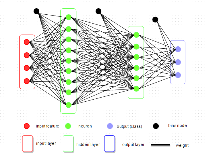
This example shows a FCN with two hidden layers. More complicated DNNs like convolutional neural networks precede the FCN with a set of convolution operations to extract features which are selected, filtered, and then used as an input layer into a final FCN for classification. We will begin our exploration of DNNs with a PyTorch example that classifies images of handwritten numbers from 0 to 9 using a simple FCN.
Neural networks, including deep neural networks, are made up of specialized perceptrons called neurons. A perceptron is an element that receives binary input(s) \(\{ x_1, \ldots, x_n \}\) and generates a binary output.

Weights \(\{ w_1, \ldots, w_n \}\) are normally applied to the inputs to define their importance. If the sum of the inputs multiplied by their weights exceeds a threshold or bias \(b_i\), the perceptron fires 1, otherwise it fires 0.
\[ \text{output} = \begin{cases} 0 \; \text{if} \; \sum_i{w_i\,x_i} \leq b_i \\ 1 \; \text{if} \; \sum_i{w_i\,x_i} > b_i \end{cases} \]We will normally simplify this notation by moving the bias inside the equation and using a dot product for the sum.
\[ \text{output} = \begin{cases} 0 \; \text{if} \; w \cdot x - b \leq 0 \\ 1 \; \text{otherwise} \end{cases} \]Bias \(b_i\) is a measure of how easy or difficult it is to make a perceptron fire. The larger \(b_i\), the more input or activation perceptron i needs to fire.
Although useful, perceptrons are inconvenient since both their inputs and outputs are binary. To address this, we normally convert perceptrons to neurons. Neurons accept continuous inputs and generate continuous outputs. To do this, neurons apply a function like sigmoid to produce smooth output over a fixed range. For example, "sigmoid" neurons accept continuous input and apply \(\sigma\) to the weighted sum of activation plus bias to produce continuous output on the range \(0, \ldots, 1\).
\[ \begin{align} z & = w \cdot x + b \\ \text{output} & = \sigma(z) = \frac{1}{1 + e^{-z}} = \frac{1}{1 + \text{exp}(-(w \cdot x + b))} \end{align} \]Intuitively, if \(z=w \cdot x + b\) is large, \(e^{-z} \approx 0\) so \(\sigma(z) \approx 1\) and if \(z\) is small \(\sigma(z) \approx 0\), just like a perceptron. The difference is that \(\sigma\) is smooth over the range \(0, \ldots, 1\) so a small change in weights or biases \(\Delta w_i\) or \(\Delta b_i\) will produce a small change in output, versus a perceptron's potential to flip its output from 0 to 1 or vice versa.
\[ \Delta \text{output} \approx \sum_i\frac{ \partial \, \text{output}}{\partial w_i} \Delta w_i + \frac{\partial \, \text{output}}{\partial b_i} \Delta b_i \]That is, \(\Delta\)output is linear in \(\Delta w\) and \(\Delta b\).
PyTorch's dataset repository includes the MNIST database of handwritten images, which includes 60,000 training examples and 10,000 test examples. It is a very common dataset to use to test learning or pattern recognition algorithms on real-world data, without the need to hand-label a large training dataset.
Normally, images are processed with CNNs. However, we will use a simple FCN to recognize the handwritten images. This is done by converting each handwritten digit image into a set of pixel values, then converting that into a one-dimensional vector. This 1D vector acts as input to one or more hidden layers, filters like ReLU (rectified linear unit), and finally to an output layer with ten possible classifications representing the ten digits 0–9. Here are two simple examples of the digits in the MNIST dataset.

In our example neural network to "learn" MNIST images we have a \(28 \times 28 = 784\)-element input vector of greyscale intensities, an \(n=15\) neuron hidden layer, and 10 output values representing a decision on which digit the input image represents. To train and validate the DNN model, MNIST provides 60,000 labeled training images and 10,000 labeled test images, denoted as \(x\) and \(y\), respectively. Any individual \(x_i\) is a 784-length vector and the corresponding \(y_i\) is a 10-length output vector with all 0s except for the target digit position, which is 1.
Our goal is to train a neural network so output approximates \(y_i = y(x_i) \, \forall x_i\) in the training set. To do this, we define a cost function to measure accuracy or error for any given prediction.
\[ C(w,b) = \frac{1}{2n} \sum_x || y(x) - a ||^{2} \]where \(w\), \(b\), \(y\), and \(a\) are weights, biases, known output vectors (labels), and predicted output vectors (activation) for all training input samples \(x\). You should recognize this as the simple quadratic function mean squared error (MSE), where \(C(w,b) \rightarrow 0\) as we improve our ability to predict correct output.
Obviously, when we start we expect \(C(w,b)\) to be large. To reduce it, we optimize \(w\) and \(b\) throughout the network using gradient descent. Ignoring for now the specifics of our neural net, how can we minimize \(C(v)\) where \(v\) are tunable parameters? For simplicity, assume \(v=(v_1,v_2)\) is a two-dimensional parameter vector. Plotting \(C(v)\) produces a valley-like image.

From any point on the valley, we want to move in a direction with the steepest slope towards the valley bottom (minimum \(C\) value). What happens when we move a small amount \(\Delta v_1\) in the \(v_1\) direction? Or a small amount \(\Delta v_2\) in the \(v_2\) direction?
\[ \Delta C \approx \frac{\partial C}{\partial v_1} \Delta v_1 + \frac{\partial C}{\partial v_2} \Delta v_2 \]We want \(C\) to be negative. Defining \(\Delta v = (\Delta v_1, \Delta v_2)^{T}\) and gradient of descent \(\nabla C =\,\)\(( \frac{\partial C}{\partial v_1}, \frac{\partial C}{\partial v_2} )\), we have
\[ \Delta C = \nabla C \cdot \Delta v \]Now, if we pick \(\epsilon\) s.t.
\[ \Delta v = -\epsilon \nabla C \]where \(\epsilon\) is the learning rate and therefore \(\Delta v\) is a small movement in the direction of steepest gradient, then
\[ \Delta C = \nabla C \cdot -\epsilon \nabla C = -\epsilon || \nabla C ||^{2} \]Since \(||\nabla C\,||^{2}\) is always positive, \(\Delta C\) is always negative. Setting \(v \rightarrow v^{\prime} = v - \epsilon \nabla C\) over and over, we will converge on a minimum \(C\), as long as \(\epsilon\) is not too big, causing us to "jump" back and forth over the minimum, or too small, causing convergence to be too expensive. Moreover, if we expand \(v\) into a vector of \(m > 2\) variables \(v=(v_1, \ldots, v_m)\), this approach continuous to work.
\[ \begin{align} \Delta C & = \nabla C \cdot \Delta v \\ \nabla C & = (\frac{\partial C}{\partial v_1}, \ldots, \frac{\partial C}{\partial v_m}) \\ \Delta v & = -\epsilon \nabla C \\ v \rightarrow v^{\prime} & = v - \epsilon \nabla C \\ \end{align} \]How do we extend this general gradient descent approach to our specific goal of optimizing \(C\) in a neural network. We simply rewrite the above equations in terms of \(w\) and \(b\).
\[ \begin{align} w_i \rightarrow w_i^{\prime} & = w_i - \epsilon \frac{\partial C}{\partial w_i} \\ b_i \rightarrow b_i^{\prime} & = b_i - \epsilon \frac{\partial C}{\partial b_i} \\ \end{align} \]We can now walk backwards through the layers in the neural network, adjusting (backpropegating) weights and biases for each neuron. To do this, recall \(C = \frac{1}{n} \sum_x C_x\) and \(C_x =\,\)\(\frac{||y_i(x_i) - a_i||^{2}}{2}\). To compute \(\nabla C\) we compute \(\Delta C_x \; \forall x\) and average the result.
\[ \nabla C = \frac{1}{n} \sum_x \nabla C_x \]If the number of neurons \(n\) is very large, we may want to sample \(\nabla C_x\). This is called stochastic gradient descent, where we randomly choose \(m \ll n\) training inputs to form a mini-batch \((x_1, \ldots, x_m)\), assuming
\[ \begin{align} \sum_{i=1}^{m} \frac{\nabla C_{x_i}}{m} & \approx \sum_x \frac{\nabla C_x}{n} = \nabla C \\ \nabla C & \approx \frac{1}{m} \sum_{i=1}^{m} \nabla C_{x_i} \\ w_i \rightarrow w_{i}^{\prime} & = w_i = \frac{\epsilon}{m} \sum_i \frac{\partial C_{x_i}}{\partial w_i} \\ b_i \rightarrow b_{i}^{\prime} & = b_i = \frac{\epsilon}{m} \sum_i \frac{\partial C_{x_i}}{\partial b_i} \\ \end{align} \]We then pick another mini-batch from the remaining samples, repeat the above process and continue until the training set is exhausted. This is defined as one training epoch.
To begin, we review and simplify the feed-forward component of DNN training to use matrix notation.
\(\therefore\) \(a_{j}^{\ell} = \sigma(\sum_k w_{jk}^{\ell} a_{k}^{(\ell-1)} + b_{j}^{\ell})\).
To convert to matrix format, define a weight matrix \(w^{\ell}\) for layer \(\ell\) where \(w^{\ell}\) are weights connecting to layer \(\ell\)'s neurons.
\[ w^{\ell} = \underbrace{ \begin{bmatrix} w^{\ell}[j,k] \\ = w_{jk}^{\ell} \end{bmatrix} }_{k\text{ input weights}} \;\;\Bigg\}\;{\scriptsize j\text{ neurons}} \]Similarly for layer \(\ell\), \(b^{\ell}\) is a bias vector with \(b_{j}^{\ell}\) the bias for neuron \(j\) in layer \(\ell\). \(a^{\ell}\) is an activation vector with \(a_{j}^{\ell}\) the activation for neuron \(j\) in layer \(\ell\).
Finally, we use vectorization to apply the activation function to weights times previous layer activations plus biases.
\[ \sigma \left( \begin{bmatrix} x_1 \\ \cdots \\ x_m \end{bmatrix} \right) = \begin{bmatrix} \sigma(x_1) \\ \cdots \\ \sigma(x_m) \end{bmatrix} \]Combining all of these, for layer \(\ell\)
\[ a^{\ell} = \sigma( w^{\ell} a^{(\ell-1)} + b^{\ell}) \]The value \(z^{\ell} = w^{\ell} a^{(\ell-1)}+b^{\ell}\) is important, so we explicitly extract it and define it as the weighted input to neurons in layer \(\ell\). We can now write
\[ \begin{align} a^{\ell} & = \sigma(z^{\ell})\\ z_{j}^{\ell} & = \sum_k w_{jk}^{\ell} a^{(\ell-1)} + b_{j}^{\ell} \end{align} \]The goal of backpropegation is to compute \(\frac{\partial C}{\partial w}\) and \(\frac{\partial C}{\partial b}\) for cost function \(C\), w.r.t. weights \(w\) and biases \(b\) in the network. To do this, we make two assumptions about \(C\). You can assume our \(C\) is MSE, \(C = \frac{1}{2n} \sum_x || y(x) - a^{L}(x)||^2\), where
For two vectors \(s\) and \(t\), the elementwise product \(s \odot t\) is \((s \odot t) = s_{j} t_{j}\), e.g.,
\[ \begin{bmatrix} 1 \\ 2 \end{bmatrix} \odot \begin{bmatrix} 3 \\ 4 \end{bmatrix} = \begin{bmatrix} 1 \cdot 3 \\ 2 \cdot 4 \end{bmatrix} = \begin{bmatrix} 3 \\ 8 \end{bmatrix} \]This is know as the Hadamard or Schur product.
At a basic level, backpropegation explains how changing \(w\) and \(b\) in a network changes \(C\). Ultimately, this requires computing \(\frac{\partial C}{\partial w_{jk}^{\ell}}\) and \(\frac{\partial C}{\partial b^{\ell}}\). To do this, we introduce an intermediate quantity \(\delta_{j}^{\ell}\), the error in neuron \(j\) in layer \(\ell\). Backpropegation computes \(\delta_{j}^{\ell}\), then relates it to \(\frac{\partial C}{\partial w_{jk}^{\ell}}\) and \(\frac{\partial C}{\partial b^{\ell}}\).
Suppose, at some neuron, we modify \(z_{j}^{\ell}\) by adding a small change \(\Delta z_{j}^{\ell}\). Now, the neuron outputs \(\sigma( z_{j}^{\ell} + \Delta z_{j}^{\ell} )\), propegating through follow-on layers in the network and changing the overall cost \(C\) by \(\frac{\partial C}{\partial z_{j}^{\ell}}\)\(\Delta z_{j}^{\ell}\). If \(\frac{\partial C}{\partial z_{j}^{\ell}}\) is large, we can improve \(C\) by choosing \(\Delta z_{j}^{\ell}\) with a sign opposite to \(\frac{\partial C}{\partial z_{j}^{\ell}}\). If \(\frac{\partial C}{\partial z_{j}^{\ell}}\) is small, though, \(\Delta z_{j}^{\ell}\) will have little impact on \(C\). Intuitively, \(\frac{\partial C}{\partial z_{j}^{\ell}}\) is a measure of the amount of error in a neuron.
Given this, we define error \(\delta_{j}^{l}\) of neuron \(j\) in layer \(\ell\) as
\[ \delta_{j}^{\ell} = \frac{\partial C}{\partial z_{j}^{\ell}} \]As before, \(\delta^{\ell}\) is a vector of errors for neurons in layer \(\ell\). Backpropegation computes \(\delta^{\ell}\) for every layer, then relates \(\delta^{\ell}\) to the quantities of real interest, \(\frac{\partial C}{\partial w_{jk}^{\ell}}\) and \(\frac{\partial C}{\partial b^{\ell}}\)
Eq 1: Computing \(\delta^{L}\) error in the output layer.
Components of \(\delta^{L}\) are
\[ \delta_{j}^{L} = \frac{\partial C}{\partial a_{j}^{L}} \sigma^{\prime}(z_{j}^{L}) \]\(\frac{\partial C}{\partial a_j^L}\) measures how fast cost is changing as a function of output activation \(j\). \(\sigma^{\prime}(z_y^L)\) measures how fast activation function \(\sigma\) is changing at \(z_y^{L}\). \(z_y^{L}\) is computed during feed-forward, so \(\sigma^{\prime}(z_y^L)\) is easily obtained. \(\frac{\partial C}{\partial a_j^L}\) depends on \(C\), but for our MSE cost function \(\frac{\partial C}{\partial a_j^L} =\,\) \((a_j^{L} - y_j)\).
To extend \(\delta_j^L\) to matrix-based form
\[ \delta^L = \nabla_a C \odot \sigma^{\prime}(z^L) \]where \(\nabla_a C\) is a vector whose components are \(\frac{\partial C}{\partial a_j^L}\). \(\nabla_a C\) expresses the rate of change of \(C\) w.r.t. output activations. In our example \(\nabla_a C = (a^L - y)\), so the full matrix form of Eq. 1 is
\[ \sigma^L = (a^L - y) \odot \sigma^{\prime}(z^L) \]Eq 2: Computing \(\delta^{\ell}\) from \(\delta^{\ell+1}\)
Given \(\delta^{\ell+1}\)
\[ \delta^{\ell} = ((w^{\ell+1})^{T} \delta^{\ell+1}) \odot \sigma^{\prime}(z^{\ell}) \]where \((w^{\ell+1})^{T}\) is the transpose of the weight matrix \(w^{\ell+1}\) for layer \(\ell+1\).
Suppose we know the error \(\delta^{\ell+1}\) at layer \(\ell+1\). Applying \((w^{\ell+1})^{T}\) moves error backwards, giving us some measure of error in layer \(\ell\). Applying the Hadamard product \(\odot \sigma^{\prime}(z^{\ell})\) pushes error backwards through the activation function in layer \(\ell\), giving us backpropegated error \(\delta^{\ell}\) in weighted input to layer \(\ell\).
We can use this to compute error \(\delta^{\ell}\) for any layer \(\ell\) by starting with \(\delta^{L}\) (Eq. 1), using it to calculate \(\delta^{L-1}\), then \(\delta^{L-2}\) and so on until \(L-i=\ell\).
Eq 3: Rate of change of \(C\) w.r.t. bias
It turns out that \(\frac{\partial C}{\partial b_j^{\ell}} =\,\) \(\delta_j^{\ell}\). That is, error \(\delta_j^{\ell}\) is exactly equal to the rate of change of bias \(\frac{\partial C}{\partial b_j^{\ell}}\). Since we already know how to compute \(\delta_j^{\ell}\), we can rewrite this as
\[ \frac{\partial C}{\partial b} = \delta \]where \(\delta\) is being evaluated at the same neuron as bias \(b\).
Eq 4: Rate of change of \(C\) w.r.t. weight
Here
\[ \frac{\partial C}{\partial w_{jk}^{\ell}} = a_k^{\ell-1} \delta_j^{\ell} \]so partial derivative \(\frac{\partial C}{\partial w_{jk}^{\ell}}\) depends on \(\delta^{\ell}\) and \(a^{\ell-1}\), which we already know how to compute. Our equation can be rewritten as
\[ \frac{\partial C}{\partial w} = a_\text{in} \delta_\text{out} \]where \(a_\text{in}\) is activation of the neuron's input to its weight \(w\) and \(\delta_\text{out}\) is the error of the neuron output for its weight \(w\). Examining just weight \(w\) and the two neurons connected by that weight

Combining all four equations, we obtain
PyTorch is, at its core, a tensor computing language with GPU acceleration support and a deep neural network library. PyTorch began as an internship program by Adam Paszke (now a Senior Research Scientist at Google) in October 2016. It was based on Torch, an open-source machine learning library and scientific computing framework written in the Lua programming language.
Three additional authors (Sam Gross, Soumith Chintala, and Gregory Chanan) formed the original author list. PyTorch was released as an open source machine learning language using the BSD open source license. Facebook currently operates both PyTorch and the Convolutional Architecture for Fast Feature Embedding (Caffe2, now part of the standard PyTorch library). It is one of the standard libraries for deep neural network research and implementation.
A basic data structure for holding data in PyTorch is a tensor. An m × n tensor is a multidimensional data structure with n rows and m columns, very similar to a Numpy ndarray. One critical difference between tensors and Numpy arrays is that tensors can be moved to the GPU for rapid processing. Below is a very simple example of creating a 2 × 2 PyTorch tensor.
If we wanted to move the tensor to the GPU, we would first check to ensure GPU processing is available, then use the to() method to transfer the tensor from CPU memory to GPU memory.
Note: If you're using a Mac with Apple silicon (M1, M2, M3,
or M4), you need to use mps as your device,
not cuda since CUDA s specific to NVIDIA GPUs.
One important caveat is that you must do all processing on either the CPU or the GPU. You cannot split data structures and processing between the two processors. So, if you move your tensors to the GPU, you must also move your DNN models to the GPU and ensure all operations are performed on the GPU.
As an initial example, we will run a simple wheat seed classifier. The dataset contains properties of three types of wheat seeds. The goal is to use these properties to predict the type of wheat the seed represents. we will first demonstrate a "from scratch" DNN that uses a simple single-layer neural network to train, then predict wheat seeds.
| Province | Area | Perimeter | Compactness | Kernel Length | Kernel Width | Assymetry | Groove Length | Type |
|---|---|---|---|---|---|---|---|---|
| Ontario | 15.26 | 14.84 | 0.871 | 5.763 | 3.312 | 2.221 | 5.22 | 1 |
| Manitoba | 14.88 | 14.57 | 0.8811 | 5.554 | 3.333 | 21.018 | 4.956 | 1 |
| Nova Scotia | 19.13 | 16.31 | 0.9035 | 6.183 | 3.902 | 2.109 | 5.924 | 2 |
| \(\cdots\) | ||||||||
The following Python-only DNN uses a simple single-layer 10-neuron DNN (ANN, actually) with a learning rate \(\epsilon=0.1\), a learning rate decay of 0.01 per epoch, 1000 training iterations per epoch, a single epoch, and five-fold cross validation during testing.
Next, we'll show the processing the same dataset, but instead of doing it in raw Python, we'll use PyTorch, Facebook's Python-based DNN library. This will demonstrate how much easier it is to use PyTorch to build a significantly more complicated DNN to train, then predict wheat types based on wheat seed properties.
The purpose of these examples is, first, to show you how to code your own DNN using basic Python, then how to use one of the most popular Python libraries (TensorFlow, programmed in C, is the other candidate) to perform the same computation in a simpler to program and more sophisticated, manner.
PyTorch's dataset repository includes the MNIST database of handwritten images, which includes 60,000 training examples and 10,000 test examples. It is a very common dataset to use to test learning or pattern recognition algorithms on real-world data, without the need to hand-label a large training dataset.
Normally, images are processed with CNNs. However, we will use a simple FCN to recognize the handwritten images. This is done by converting each handwritten digit image into a set of pixel values, then converting that into a one-dimensional vector. This 1D vector acts as input to a single hidden layer, an ReLU (rectified linear unit) filter, and an output layer with ten possible classifications representing the ten digits 0–9. Here are two simple examples of the digits in the MNIST dataset.
Here is a Jupyter Notebook we will use to load the MNIST dataset, construct a simple FCN, then train and test it on the MNIST data.
Even with a simple FCN with a single hidden layer and an ReLU filter, five training epochs (evaluating the training dataset five times) produces results of 97% or better on the test dataset.
To see how well an FCN works on real two-dimensional images, we will work with the CIFAR10 dataset, also a part of PyTorch's dataset repository. CIFAR10 contains 50,000 training images and 10,000 test images of size \(32 \times 32 \times 3\): 32 pixels wide by 32 pixels high by 3 pixel components R (red), G (green), and B (blue).
Note the classes variable. This is used to convert the
label value for an image into a semantic text description of the class
it belongs to. You will probably want to define this and index into it
to better understand which classes the images belong to.
If you want to examine some of the images in the CIFAR10 dataset, you can modify the code in our original FCN example. However, a simpler way to do this and show more images would be as follows.

Apart from changing any occurrences 28 * 28 to 32
* 32 * 3 (to account for the different input size), the
remainder of the code can be identical to the MNIST FCN. You're
certainly encouraged to also vary things like
criteria, optimizer, hidden_size,
the number of hidden layers, and other properties of the FCN to try to
improve performance. Remember that, for ten classes, just like the
MNIST dataset, chance is 10%. You're unlikely to obtain accuracies
anywhere near the 97% we produce for the MNIST images, but you should
be able to do much better than 10%, even for this most simple FCN.
Here is a simple Jupyter Notebook that trains on the CIFAR10 dataset using our simple FCN.
The wheat dataset is fairly easy to process, but it is probably more representative of the type of task you need to solve: classification from one or more input properties. DNNs themselves have been applied most successfully to image data using convolutional neural networks (CNNs). A CNN converts an \(n \times m\) image to an \(nm\) vector, then uses that vector as input into a convolution stage. Here, a collection of \(k\) kernels are convolved against the pixels and their immediate neighbours to produce scalar values. For each kernel, a column of \(nm\) convolved values are created, one for each pixel in the image. In the simplest CNN, the column values are evaluated to produce a single, representative value. For example, max scans a column and extracts the largest value. These values form a \(k\)-length input vector to a follow-on fully connected network. This network processes output from the CNN to generate a final classification prediction.
Convolutional neural networks (CNNs) extend FCNs by preceding the fully connected layers with a set of convolutional layers. CNNs are commonly used to analyze images, although recent research has shown that they can handle other data modalities like text with excellent performance.
CNNs are made up of a number of standard operations to produce new, hidden layers. These include
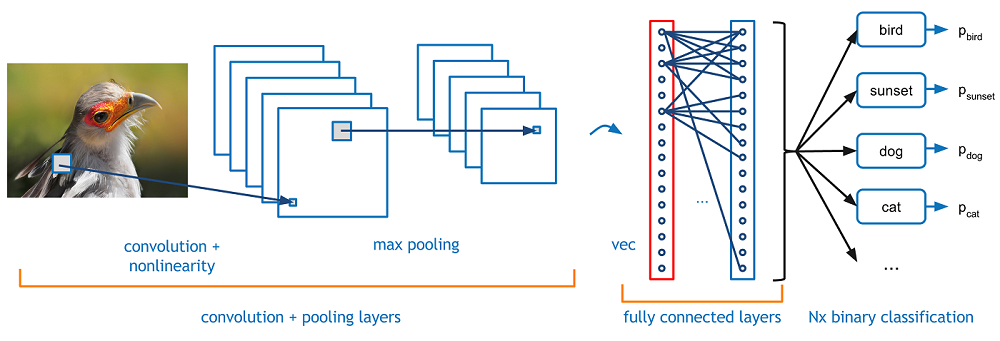
In practice, it is common to apply a series of CONV-RELU layers, follow them with a POOL layer, and repeat this pattern until an image has been processed to a small size. At this point, results are formed into a 1D vector which acts as input to an FCN. The FCN produces a set of probabilities for each possible classification (softmax).
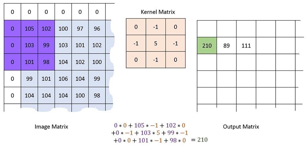
Convolution combines a pixel in an image and its neighbours by placing a kernel of a given size centered over the pixel, then multiplying the corresponding pixel and kernel values, and summing them together to produce a final filtered result.
The example above using a 3×3 kernel with values -1, 0, and 5 at various positions within its nine cells. When we center it over the pixel at the center of the purple box, multiple, and sum, we obtain a final filtered value of 210 for that position in the image. Kernels are designed to identify specific properties of an image, producing large values when those properties are located, and small values when they are not. For example, the Kirsch filter is designed to identify edges in an image. Convolution of a simple animation with a Kirsch filter produces the result shown below.

|
|
||||||||||||

|
|||||||||||||
Normally, we use numerous kernels to identify different properties or features in an image. Each kernel produces a feature map from the image. These feature maps are normally stacked one on top of another, producing a result with width and height one less than the original image size, and depth equal to the number of kernels applied to the image. How does the CNN decide on the kernel values for each kernel? This occurs during training. Kernel values are initially random, and slowly converge along with edge weights during backpropagation to identify image properties salient to classifying the images.
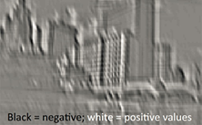
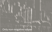
Filtering adjusts values in a feature map, for example, by normalizing them, or by removing negative values. The common ReLU filter, for example, removes negative values and retains positive values.
|
|
|
Pooling takes a feature map, and reduces its size by aggregating block of values. Aggregation can use any common mathematical operator like average, median, maximum or minimum. Pooling uses a window size which defines its width and height, and a stride which defines the step size it uses as it slides over the feature map values it pools.

|
max pooling → 2×2 window → stride 2 |

|
Recall in the previous discussion of FCNs, we used the MNIST handwriting image dataset. We are now switching to the CIFAR10 dataset of photographic images. In your exercise, you were asked to re-purpose the FCN to handle images from CIFAR10. Here is a simple Jupyter Notebook that does that.
Although this produces results better than chance, we can further improve performance by using a simple CNN.
Results for the CNN are indeed better than the FCN, but only by a few percentage points. This suggests the CNN could be improved possibly significantly, by expanding the CONV/RELU/POOL part of the image to better capture the features needed to differentiate different image classes from one another. One clue is in the individual class accuracies, which show that natural images like cats and deer are being labeled much less accurately than man-made images like cars and trucks.