[ Home Page ] [ CSC Home Page ] [ NCSU Home Page ]
Note: Work described within is a summary of a paper that was published in Proceedings Graphics Interface 2000; a PDF version is available for downloading.
Oriented Texture Slivers: A Technique for Local Value Estimation of Multiple Scalar Fields
Chris Weigle, William Emigh, Geniva Liu, Russell M. Taylor II, James T. Enns, Christopher G. Healey
Abstract
This paper describes a texture generation technique that combines orientation and luminance to support the simultaneous display of multiple overlapping scalar fields. Our orientations and luminances are selected based on psychophysical experiments that studied how the low-level human visual system perceives these visual features. The result is an image that allows viewers to identify data values in an individual field, while at the same time highlighting interactions between different fields. Our technique supports datasets with both smooth and sharp boundaries. It is stable in the presence of noise and missing values. Images are generated in real-time, allowing interactive exploration of the underlying data. Our technique can be combined with existing methods that use perceptual colours or perceptual texture dimensions, and can therefore be seen as an extension of these methods to further assist in the exploration and analysis of large, complex, multidimensional datasets.
CR Categories: H.5.2 [Information Interfaces and Presentation]: User Interfaces - ergonomics, screen design, theory and methods; I.3.6 [Computer Graphics]: Methodology and Techniques - ergonomics, interaction techniques; J.2 [Physical Sciences and Engineering]: Physics
Keywords: computer graphics, human vision, luminance, multidimensional, orientation, perception, texture, scientific visualization
Introduction
This paper describes a new texture generation technique designed to allow rapid visual exploration and analysis of multiple overlapping scalar fields. Our technique falls in the area of scientific visualization, the conversion of collections of strings and numbers (called datasets) into images that viewers can use to "see" values, structures, and relationships embedded in their data. A multidimensional dataset contains a large number of data elements, where each element encodes n separate attributes A_1, ..., A_n. For example, a weather dataset is made up of data elements representing weather station readings. Each element encodes a latitude, longitude, and elevation, a time and date readings were taken, and environmental conditions like temperature, pressure, humidity, precipitation, wind speed, and wind direction. An open problem in scientific visualization is the construction of techniques to display data in a multidimensional dataset in a manner that supports effective exploration and analysis [McC87, Smi98].
Previous work on this problem has suggested selecting n visual features (e.g., spatial location, hue, luminance, size, contrast, directionality, or motion) to represent each of the n attributes embedded in the dataset. Although this technique can work well in practice, a number of limitations need to be considered:
- dimensionality: as the number of attributes n in the dataset grows, it becomes more and more difficult to find additional visual features to represent them.
- interference: different visual features will often interact with one another, producing visual interference; these interference effects must be controlled or eliminated to guarantee effective exploration and analysis.
- attribute-feature matching: different visual features are best suited to a particular type of attribute and analysis task; an effective visualization technique needs to respect these preferences.
The weather dataset (and numerous other practical applications) can be viewed as a collection of n scalar fields that overlap spatially with one another. Rather than using n visual features to represent these fields, we use only two: orientation and luminance. For each scalar field (representing attribute A_i) we select a constant orientation o_i; at various spatial locations where a value a_i in A_i exists, we place a corresponding sliver texture oriented at o_i. The luminance of the sliver texture depends on a_i: the maximum a_max in A_i produces a white (full luminance) sliver, while the minimum a_min in A_i produces a black (zero luminance) sliver. A perceptually-balanced luminance scale running from black to white is used to select a luminance for an intermediate value a_i, a_min < a_i < a_max (this scale was built to correct for the visual system’s approximately logarithmic response to variations in luminance [Int92]).
| 0 |
0 |
0 |
1 |
0 |
0 |
0 |
0 |
2 |
0 |
0 |
0 |
0 |
1 |
4 |
1 |
3 |
2 |
3 |
4 |
 |
| 0 |
0 |
0 |
0 |
1 |
0 |
1 |
0 |
0 |
0 |
0 |
0 |
0 |
0 |
3 |
4 |
6 |
3 |
4 |
5 |
| 0 |
0 |
0 |
0 |
0 |
1 |
0 |
1 |
0 |
1 |
0 |
0 |
0 |
1 |
0 |
7 |
5 |
6 |
4 |
6 |
| 0 |
0 |
0 |
0 |
0 |
0 |
0 |
0 |
0 |
0 |
0 |
0 |
0 |
0 |
2 |
7 |
6 |
3 |
5 |
7 |
| 0 |
1 |
0 |
1 |
1 |
1 |
0 |
9 |
9 |
1 |
0 |
0 |
0 |
0 |
0 |
6 |
5 |
7 |
0 |
1 |
| 0 |
0 |
0 |
0 |
0 |
0 |
13 |
13 |
15 |
0 |
0 |
0 |
0 |
0 |
1 |
1 |
5 |
0 |
0 |
0 |
| 0 |
0 |
0 |
1 |
0 |
15 |
16 |
15 |
16 |
18 |
0 |
0 |
0 |
0 |
0 |
0 |
0 |
0 |
0 |
0 |
| 0 |
0 |
0 |
0 |
0 |
18 |
19 |
18 |
16 |
18 |
19 |
0 |
0 |
0 |
0 |
1 |
0 |
0 |
0 |
0 |
| 0 |
0 |
0 |
0 |
0 |
16 |
19 |
20 |
20 |
19 |
16 |
0 |
1 |
0 |
0 |
0 |
0 |
0 |
0 |
0 |
| 0 |
0 |
0 |
0 |
0 |
16 |
18 |
18 |
19 |
20 |
15 |
0 |
1 |
0 |
1 |
0 |
0 |
0 |
0 |
0 |
| 1 |
0 |
0 |
0 |
15 |
17 |
17 |
18 |
17 |
19 |
19 |
0 |
5 |
0 |
0 |
0 |
0 |
0 |
0 |
0 |
| 0 |
0 |
0 |
0 |
14 |
14 |
12 |
0 |
13 |
16 |
9 |
8 |
9 |
0 |
0 |
0 |
1 |
0 |
0 |
0 |
| 0 |
0 |
0 |
9 |
12 |
13 |
14 |
0 |
0 |
14 |
10 |
7 |
0 |
1 |
1 |
0 |
0 |
0 |
0 |
0 |
| 0 |
0 |
0 |
9 |
11 |
13 |
0 |
0 |
0 |
12 |
8 |
7 |
1 |
0 |
1 |
0 |
0 |
0 |
1 |
0 |
| 0 |
0 |
7 |
8 |
9 |
0 |
0 |
0 |
0 |
10 |
9 |
0 |
0 |
0 |
0 |
0 |
0 |
0 |
0 |
0 |
| 0 |
2 |
5 |
6 |
8 |
0 |
0 |
0 |
0 |
0 |
0 |
0 |
0 |
0 |
0 |
0 |
0 |
0 |
0 |
0 |
| 0 |
3 |
4 |
5 |
6 |
0 |
0 |
0 |
1 |
0 |
0 |
0 |
0 |
0 |
0 |
0 |
0 |
0 |
0 |
0 |
| 2 |
0 |
4 |
2 |
4 |
0 |
0 |
0 |
0 |
0 |
0 |
0 |
0 |
1 |
0 |
0 |
0 |
0 |
0 |
0 |
| 2 |
1 |
2 |
4 |
0 |
0 |
0 |
0 |
0 |
0 |
0 |
0 |
0 |
0 |
0 |
0 |
0 |
0 |
0 |
0 |
| 0 |
0 |
2 |
0 |
0 |
0 |
1 |
0 |
0 |
0 |
0 |
0 |
0 |
0 |
0 |
0 |
0 |
0 |
0 |
0 |
| (a) |
|
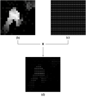
Figure 1: (a) a 20 x 20 patch of values from a scalar field; (b) the patch represented by greyscale swatches; (c) a collection of slivers oriented 0-degrees at each data value location; (d) the greyscale map and slivers are combined to produce the final sliver layer
Figure 1a shows a uniformly-sampled 20 x 20 patch from a hypothetical scalar field. Values in the field are represented as greyscale swatches in Figure 1b. A constant orientation of 0-degrees is used to represent values in the field (slivers rotated 0-degrees are placed at the spatial locations for each reading in the field, shown in Figure 1c). Blending these two representations together produces the final image (Figure 1d), a layer of variable-luminance slivers showing the positions and values of all the data in the original field.
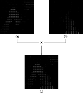
Figure 2: (a,b) two scalar fields represented with 0-degrees and 90-degrees, respectively; (c) both fields shown in a single image, overlapping values show as elements that look like plus signs
Multiple scalar fields are displayed by compositing their sliver layers together. Figure 2a-b shows two separate sliver layers representing two scalar fields. The first field uses slivers oriented 0-degrees; the second uses slivers oriented 90-degrees. When a viewer visualizes both fields simultaneously, the sliver layers are overlayed to produce the single image shown in Figure 2c. This image allows the viewer to locate values in each individual field, while at the same time identifying important interactions between the fields. The use of thin, well separated slivers is key to allowing values from multiple fields to show through in a common spatial location. A viewer can use these images to:
- determine which fields are prominent in a region,
- determine how strongly a given field is present,
- estimate the relative weights of the field values in the region, and
- locate regions where all the fields have low, medium, or high values.
We continue with a discussion of related work, focusing in particular on the use of texture patterns for multidimensional data display. Next, we describe the psychophysical experiments we used to determine how to select perceptually salient orientations. Although our visualization technique is applicable to a wide range of practical applications, we were originally motivated by a specific problem: the display of multiple atomic surface properties measured with a scanning electron microscope. We conclude by showing how our technique can be used to visualize datasets from this domain.
Related Work
Several techniques exist for displaying multidimensional datasets on an underlying surface or height field. A good overview of some of these techniques is presented in Keller and Keller [Kel91]. Our work is most similar to methods that use textures or glyphs to represent multiple attribute values at a single spatial location. We therefore focus our study of previous work on this broad area.
Texture has been studied extensively in the computer vision, computer graphics, and cognitive psychology communities. Although each group focuses on separate tasks (e.g., texture segmentation and classification, information display, or modelling the human visual system), they each need ways to describe precisely the textures being identified, classified, or displayed. Statistical methods and perceptual techniques are both used to analyse texture [Ree93]. Our focus in this paper is on identifying and harnessing the perceptual features that make up a texture pattern. Experiments conducted by Julész led to the texton theory [Jul84], which suggests that early vision detects three types of texture features (or textons): elongated blobs with specific visual properties (e.g., colour or orientation), ends of line segments, and crossings of line segments. Tamura et al. [Tam78] and Rao and Lohse [Rao93] identified texture dimensions by conducting experiments that asked subjects to divide pictures depicting different types of textures (Brodatz images) into groups. Tamura et al. used their results to propose methods for measuring coarseness, contrast, directionality, line-likeness, regularity, and roughness. Rao and Lohse applied multidimensional scaling to identify the primary texture dimensions used by their subjects to group images: regularity, directionality, and complexity. Haralick et al. [Har73] built greyscale spatial dependency matrices to identify features like homogeneity, contrast, and linear dependency. Liu and Picard [Liu94] used Wold features to synthesize texture patterns. A Wold decomposition divides a 2D homogeneous pattern (e.g., a texture pattern) into three mutually orthogonal components with perceptual properties that roughly correspond to periodicity, directionality, and randomness.
Work in computer graphics has studied methods for using texture patterns to display information during visualization. Grinstein et al. [Gri89] built "stick-men" icons to produce texture patterns that show spatial coherence in a multidimensional dataset. Ware and Knight [War95] used Gabor filters to construct texture patterns; attributes in an underlying dataset are used to modify the orientation, size, and contrast of the Gabor elements during visualization. Turk and Banks [Tur96] described an iterated method for placing streamlines to visualize two-dimensional vector fields. Interrante [Int97] displayed texture strokes to help show three-dimensional shape and depth on layered transparent surfaces. Healey and Enns [Hea98, Hea99] described perceptual methods for measuring and controlling perceptual texture dimensions during multidimensional visualization. van Wijk [van91], Cabral and Leedom [Cab93], and Interrante and Grosch [Int98] used spot noise and line integral convolution to generate texture patterns to represent an underlying flow field. Finally, Laidlaw described painterly methods for visualizing multidimensional datasets with up to seven values at each spatial location [Kir99, Lai98].
Our technique is perhaps most similar to the stick-man method used in EXVIS [Gri89], or to the pexels (perceptual texture elements) of Healey and Enns [Hea98, Hea99]. EXVIS shows areas of coherence among multiple attributes by producing characteristic texture patterns in these areas. We extend this technique by allowing a viewer to estimate relative values within an individual field, while still producing the characteristic textures needed to highlight interactions between different fields.
Orientation Categories
In order to effectively represent multiple scalar fields with different orientations, we need to know how the visual system distinguishes between orientations. In simple terms, we want to determine whether the visual system differentiates orientation using a collection of perceptual orientation categories. If these categories exist, it might suggest that the low-level visual system can rapidly distinguish between orientations that lie in different categories.
Psychophysical research on this problem has produced a number of interesting yet incomplete conclusions. Some researchers believe only three categories of orientation exist: flat, tilted, and upright [Wol92]. Others suggest a minimum rotational difference d is necessary to perceive a spatial collection of target elements oriented tg in a field of background elements oriented bg (i.e., d = | tg - bg |). More recent work has shown that d is dependent on bg [Not85, Not91]. For example, if the background elements are oriented 0-degrees (i.e., horizontal or flat), only a small rotation may be needed to differentiate a group of target elements (e.g., tg = 10-degrees and d = tg - bg = 10-degrees). On the other hand, a much larger rotational difference might be necessary to distinguish a target group in a sea of background elements oriented 20-degrees (e.g., tg = 40-degrees and d = tg - bg = 20-degrees). Based on these results, we seek to construct a function f(bg) that will report the amount of rotational difference d needed to perceive a group of target elements oriented tg = bg + d in a sea of background elements oriented bg.
Experimental Design
We began our investigation by attempting to construct a discrete function f(bg) for 19 different background orientations of 0, 5, 10, ..., 90-degrees. The function f returns rotational differences in 5-degree intervals (e.g., d = 5-degrees, d = 10-degrees, d = 15-degrees, and so on). Our experiment was designed to answer the following questions:
- In a sea of background elements oriented bg, how much counterclockwise rotation d_ccw is needed to differentiate a group of target elements oriented tg = bg + d_ccw?
- How much clockwise rotation d_cw is needed to differentiate a group of target elements oriented at tg = bg - d_cw?
- For a given background bg, do d_ccw and dcw differ significantly?
- Do certain backgrounds (e.g., the cardinal directions 0, 45, and 90-degrees) have significantly lower d_ccw or d_cw?
- What is the maximum number of rapidly distinguishable orientations we can construct in the range 0-90-degrees?
The initial experiment was divided into two parts: one to test background orientations from 0-45-degrees, the other to test background orientations 45-90-degrees. We describe trials in the 0-45-degree experiment. Apart from the specific orientations used, the design of the 45-90-degree experiment was identical.
During the experiment the background orientation was increased in 5-degree steps from 0-degrees to 45-degrees. This resulted in 10 different background subsections (0, 5, 10, ..., 45-degrees). Every possible target orientation was tested for each separate background. For example, targets oriented 5, 10, 15, 20, 25, 30, 35, 40, and 45-degrees were tested in a sea of background elements oriented 0-degrees. Targets oriented 0, 5, 10, 20, 25, 30, 35, 40, and 45-degrees were tested in a sea of background elements oriented 15-degrees.
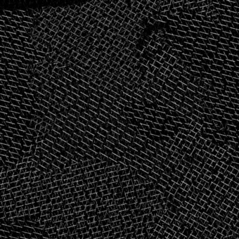
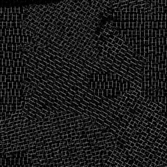
Figure 3: An example of three experiment displays: (a) a 10-degree target in a 0-degree background (target is five steps right and seven steps up from the lower left corner of the array); (b) a 30-degree background with no target; (c) a 65-degree target in a 55-degree background (target is six steps left and seven steps up from the lower right corner of the array)
A total of 540 trials were run during the experiment (six for each of the 90 different background/target pairs). Each trial contained a total of 400 rectangles arrayed on a 20 x 20 grid. The position of each rectangle was randomly jittered to introduce a measure of irregularity. Three trials for each background/target pair contained a 2 x 2 target patch (as in Figure 3a, c); the other three did not (as in Figure 3b). Twenty undergraduate psychology students were randomly selected to participate during the experiment (ten for the 0-45-degree experiment and ten for the 45-90-degree experiment). Subjects were asked to answer whether a target patch with an orientation different from the background elements was present or absent in each trial. They were told that half the trials would contain a target patch, and half would not. Subjects were instructed to answer as quickly as possible, while still trying to maintain an accuracy rate of 90% or better. Feedback was provided after each trial to inform subjects whether their answer was correct. The entire experiment took approximately one hour to complete. Subject accuracies (1 for a correct answer, 0 for an incorrect answer) and response times (automatically recorded based on the vertical refresh rate of the monitor) were recorded after each trial for later analysis.
Results
Mean subject response times rt and mean subject error rates e were used to measure performance. A combination of multi-factor analysis of variance (ANOVA) and least-squares line fitting showed:
- A target oriented d = +/-15-degrees or more from its background elements resulted in the highest accuracies and the fastest response times, regardless of background orientation.
- e for backgrounds oriented 0 or 90-degrees was significantly lower than for the other backgrounds.
- e for targets oriented 0 or 90-degrees was significantly higher than for the other targets, suggesting an asymmetry (good as a background, bad as a target) for these orientations.
- There were no systematic differences in either e or rt between clockwise and counterclockwise rotations about any background orientation.
- There was no significant difference in e between the 0-45-degree and the 45-90-degree experiments for corresponding background/target pairs, however, within the range rt was slower during the 45-90-degree experiment, compared to the 0-45-degree experiment.
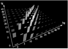
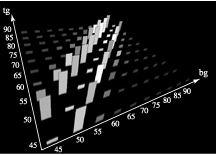
Figure 4: (a) results for the 0-45-degree experiment, one strip for each background/target pair; the height of the strip represents e (taller for more errors), the brightness of the strip represents rt (brighter for longer response times); locations where bg = tg (the diagonals on each graph) represent target absent trials; (b) results for the 45-90-degree experiment
Regardless of the specific background orientation being displayed, any target oriented d = +/-15-degrees or more from the background produced near-perfect accuracy and fast response times (F(1, 90) = 8.06, p < 0.01 and F(1, 90) = 2.96, p < 0.05 for e and rt, respectively, in the d = +/-15-degree range). This suggests that any target with an absolute rotational difference of 15-degrees or more from the background can be rapidly and accurately perceived.
When background elements were oriented 0 or 90-degrees, targets were detected more accurately (F(9, 810) = 12.82, p < 0.001 at d = 5-degrees). On the other hand, targets oriented 0 or 90-degrees were detected less accurately (e.g, a 90-degree target in a background of elements rotated 85 or 80-degrees, or a 0-degree target in a background of elements rotated 5 or 10-degrees; F(1, 162) = 48.02, p < 0.001 at d = 5-degrees; F(1, 162) = 29.91, p < 0.001 at d = 10-degrees). This orientation asymmetry is documented in the psychophysical literature [Tri88, Tri91]. In terms of visualization, it suggests we should treat the cardinal directions 0 and 90-degrees carefully; although they produce less visual interference (i.e., they act well as background orientations), they can be significantly more difficult to detect (i.e., they act poorly as target orientations).
We found a small but statistically significant increase in rt during the 45-90-degree experiment (F(1, 90) = 6.08, p < 0.05 over the d = +/-10-degree range, shown by brighter strips in Figure 4b). Since the overall pattern of response times between the two experiments is identical, we believe this result is due to a difference between subjects (i.e., subjects in the 45-90-degree experiment simply needed more time to feel comfortable about the answers they gave). Even if the results are significant for all viewers, the small differences we encountered would not be important for applications that allow a viewer to spend time exploring an image. However, these differences could be important in real-time environments or during long viewing sessions. Additional experiments are needed to determine if any real differences in response times exist.
Two additional findings allow us to simplify our selection of orientations. First, there were no systematic differences in either e or rt between clockwise and counterclockwise rotations about any background orientation. In three cases (backgrounds of 55, 65, and 70-degrees) clockwise rotations were significantly faster; in two other cases (backgrounds of 25 and 30-degrees) counterclockwise rotations were significantly faster. Since subjects did not exhibit a consistent preference for either direction, we concluded that we can rotate the same amount in either direction to make a target patch salient from its background elements. Finally, there was no significant difference in e between the 0-45-degree experiment and the 45-90-degree experiment (F(1, 18) = 0.157, p = 0.6893). This means that, given a reasonable amount of time to search, accuracy in each set of backgrounds is statistically equal, and the two ranges can be considered mirror images of one another.
We conclude by noting that our experiments investigated how to distinguish multiple orientations from one another. This is a first step towards determining how many orientations the visual system can identify simultaneously (i.e., the ability to identify the presence or absence of a sliver with a specific orientation). Our results provide a solid foundation from which to build future experiments that study the question "How many different orientations can I identify from one another?"
Emergent Features
An overlap between high-value regions in different scalar fields appears as a collection of slivers sharing common spatial locations. The overlapping slivers form shapes like plus, X, or star. It is often critical for viewers to be able to identify these overlapping regions. Although we did not conduct experiments on the perceptual salience of each type of overlap, the shapes they form fall into the broad category of emergent features [Pom89]. An emergent feature is created by grouping several simpler shapes together. Although emergent features cannot always be predicted by examining the simpler shapes in isolation, they result in perceptually salient visual properties like intersection, closure, and shape (or curvature). We believe that all of the overlapping sliver types will produce at least one emergent feature (e.g., every overlap will produce an intersection between the slivers). The emergent features make the locations of the overlapping regions salient from neighbouring, non-overlapping areas.
Implementation
Figure 1 shows the general process for creating one sliver layer. The slivers in Figure 1 are positioned on an underlying regular grid. In practice, however, we must jitter the placement of each sliver. This helps to prevent the technique from imposing any strong artificial structure on the data. Separating the slivers is also necessary to allow multiple slivers with different orientations to show through at common spatial locations. The base texture used to make the images in this paper is 10% sliver, 90% empty. We employed the image-guided streamline placement package of Turk and Banks [Tur96] on a constant vector field to generate the base texture. Since we viewed this as a pre-processing step, the time used to build the base texture was not a critical concern.
Next, we assign an orientation to each scalar field in the dataset. Since slivers oriented 0-180-degrees are mirror images of slivers rotated 180-360-degrees, we restricted our selections to the 0-180-degree range. During implementation we assumed the experimental results from our 0-90-degree range were identical for orientations covering 90-180-degrees. Anecdotal findings during the use of our system suggest this assumption is valid. We can immediately obtain 13 separate orientations by simply using a constant difference d = 15-degrees. If we choose to treat the cardinal directions 0-degrees and 180-degrees as special background cases that only require targets with 5-degrees of rotational difference, we can increase the number of separate orientations to 15.
Once an easily distinguishable orientation is assigned to each scalar field, the sliver layers can be constructed. The values in each field modulate the intensity of the slivers in the field’s layer. In order to avoid an obvious artifact in the center of the final image, the centers of rotation for every layer are different. We accomplish this by translating each layer’s texture centers to different points on a uniform grid. The layers are then overlayed on top of one another. The final texture is the per-pixel maximum of the overlapping sliver layers (using the maximum avoids highlights produced by averaging or summing overlapping luminances values).
We create only one base texture, rotating and translating it to form the other orientations. Alternatively, we could produce a separate base texture for each scalar field. The use of multiple base textures would prevent the appearance of regions with similar orientation-independent structures. Since we did not notice this phenomena in practice, we chose not to address this problem. Using a single base texture allows our technique to generate a 256 x 256 image with nine scalar fields at nine frames per second on a workstation with eight R10000 processors.
Practical Applications
Figure 5: (a) eight sliver layers representing calcium (15-degrees), copper (30-degrees), iron (60-degrees), magnesium (75-degrees), manganese (105-degrees), oxygen (120-degrees), sulphur (150-degrees), and silicon (165-degrees); (b) all eight layers blended into a single image; (c) silicon and oxygen re-oriented at 90-degrees and 180-degrees, respectively, to highlight the presence of silicon oxide (as a "plus sign" texture) in the upper right, upper left, and lower left corners of the image
The application for which this technique was originally developed is the display of multiple data fields from a scanning electron microscope (SEM). Each field represents the concentration of a particular element (oxygen, silicon, carbon, and so on) across a surface. Physicists studying mineral samples need to determine what elements make up each part of the surface and how those elements mix. By allowing the viewer to see the relative concentrations of the elements in a given area, our technique enables recognition of composites more easily than side-by-side comparison, especially for situations where there are complex amalgams of materials.
Figure 5a shows sliver layers representing eight separate elements: calcium (15-degrees), copper (30-degrees), iron (60-degrees), magnesium (75-degrees), manganese (105-degrees), oxygen (120-degrees), sulphur (150-degrees), and silicon (165-degrees). The orientations for each layer were chosen to ensure no two layers have an orientation difference of less than 15-degrees. Figure 5b shows the eight layers blended together to form a single image. Figure 5c changes the orientations of silicon and oxygen to 90-degrees and 180-degrees, respectively, to investigate a potential interaction between the two (the presence of silicon oxide in the upper right, upper left, and lower left where regions of "plus sign" textures appear).
Conclusions and Future Work
This paper describes a technique for using orientation and luminance to visualize multiple overlapping scalar fields simultaneously in a single image. Values in each field are represented by sliver textures oriented at a fixed rotation . A sliver’s luminance is selected based on the relative strength of the scalar field at the sliver’s spatial location. We conducted psychophysical experiments to study how the low-level human visual system perceives differences in orientation. This knowledge was used to choose orientations for each field that were easy to distinguish. Our results suggest up to 15 orientations in the 0–180-degree range can be rapidly and accurately differentiated. The greyscale ramp used to assign a luminance to each sliver was also constructed to be perceptually linear. The result is an image that shows data values in each individual field, while at the same time highlighting important interactions between the fields.
Our technique varies a sliver’s luminance, leaving chromaticity (hue and saturation) free for other uses. For example, an isoluminant, medium-intensity colour background will highlight slivers with high or low field values. If many fields have common values in the same spatial region, we can help to identify their individual boundaries by displaying some of the fields using colour. Important fields can be shown in colour rather than greyscale to further enhance their distinguishability. Recent work in our laboratory has successfully combined sliver textures with perceptual colour selection techniques, thereby increasing the amount of information we can represent in a single display.
Orientation has been identified as a perceptual texture dimension, a fundamental property of an overall texture pattern. We can vary other perceptual texture dimensions of each sliver (e.g., their size or density) to encode additional data values. We want to note that we are forming a single texture pattern by varying its underlying texture dimensions. It is not possible to overlay multiple texture patterns (e.g., spot noise and slivers) to visualize multiple data attributes; in fact, the inability to analyse texture patterns displayed on top of one another was one of the original motivations for this work.
Finally, this paper focuses on 2D orientation. Future work will study the use of 3D orientation. The first question of interest is: "Which 3D orientation properties are perceptually salient from one another?" Research in the psychophysical community has started to address exactly this question. Once these properties are identified, we can conduct experiments to test their ability to encode information, both in isolation and in combination with one another. Three-dimensional orientation properties may allow us to represent 3D scalar volumes as clouds of oriented slivers in three-space. As with 2D slivers, we want to investigate the strengths and limitations of this type of technique vis-a-vis traditional methods of volume rendering and volume visualization.
Bibliography
| Cab93 |
Cabral, B. and Leedom, L. C. Imaging vector fields using line integral convolution. In SIGGRAPH 93 Conference Proceedings (Anaheim, California, 1993), pp. 263–270. |
| Gri89 |
Grinstein, G., Pickett, R., and Williams, M. EXVIS: An exploratory data visualization environment. In Proceedings Graphics Interface ’89 (London, Canada, 1989), pp. 254–261. |
| Har73 |
Haralick, R. M., Shanmugam, K., and Dinstein, I. Textural features for image classification. IEEE Transactions on System, Man, and Cybernetics SMC-3, 6 (1973), 610–621. |
| Hea98 |
Healey, C. G. and Enns, J. T. Building perceptual textures to visualize multidimensional datasets. In Proceedings Visualization ’98 (Research Triangle Park, North Carolina, 1998), pp. 111–118. |
| Hea99 |
Healey, C. G. and Enns, J. T. Large datasets at a glance: Combining textures and colors in scientific visualization. IEEE Transactions on Visualization and Computer Graphics 5, 2 (1999), 145–167. |
| Int97 |
Interrante, V. Illustrating surface shape in volume data via principle direction-driven 3D line integral convolution. In SIGGRAPH 97 Conference Proceedings (Los Angeles, California, 1997), pp. 109–116. |
| Int98 |
Interrante, V. and Grosch, C. Visualizing 3D flow. IEEE Computer Graphics & Applications 18, 4 (1998), 49–53. |
| Int92 |
Interrante, V., Ferwerda, J., Gossweiler, R., Healey, C. G. and Rheingans, P. Applications of Visual Perception in Computer Graphics. SIGGRAPH 98 Course 32 (Orlando, Florida, 1992). |
| Jul84 |
Julesz, B. A brief outline of the texton theory of human vision. Trends in Neuroscience 7, 2 (1984), 41–45. |
| Kel91 |
Keller, P. and Keller, M. Visual cues: Practical data visualization. IEEE Computer Society Press, Los Alamitos, California, 1991. |
| Kir99 |
Kirby, R. M., Marmanis, H., and Laidlaw, D. H. Visualizing multivalued data from 2D incompressible flows using concepts from painting. In Proceedings Visualization ’99 (San Francisco, California, 1999), pp. 333–340. |
| Lai98 |
Laidlaw, D. H., Ahrens, E. T., Kremers, D., Awalos, M. J., Jacobs, R. E., and Readhead, C. Visualizing diffuse tensor images of the mouse spinal cord. In Proceedings Visualization ’98 (Research Triangle Park, North Carolina, 1998), pp. 127–134. |
| Liu94 |
Liu, F. and Picard, R. W. Periodicity, directionality, and randomness: Wold features for perceptual pattern recognition. In Proceedings 12th International Conference on Pattern Recognition (Jerusalem, Israel, 1994), pp. 1–5. |
| McC87 |
McCormick, B. H., DeFanti, T. A., and Brown, M. D. Visualization in scientific computing—A synopsis. Computer Graphics & Applications 7, 7 (1987), 61–70. |
| Nor85 |
Nothdurft, H-C. Orientation sensitivity and texture segmentation in patterns with different line orientations. Vision Research 25 (1985), 551–560. |
| Nor91 |
Nothdurft, H-C. Texture segmentation and pop-out from orientation contrast. Vision Research 31, 6 (1991), 1073–1078. |
| Pom89 |
Pomerantz, J. R. and Pristach, E. A. Emergent features, attention, and perceptual glue in visual form attention. Journal of Experimental Psychology: Human Perception & Performance 15, 4 (1989), 635–649. |
| Rao93 |
Rao, A. R. and Lohse, G. L. Identifying high level features of texture perception. Computer Vision, Graphics, and Image Processing: Graphical Models and Image Processing 55, 3 (1993), 218–233. |
| Ree93 |
Reed, T. R. and Hans Du Buf, J. M. A review of recent texture segmentation and feature extraction techniques. Computer Vision, Graphics, and Image Processing: Image Understanding 57, 3 (1993), 359–372. |
| Smi98 |
Smith, P. H. and Van Rosendale, J. Data and visualization corridors report on the 1998 CVD workshop series. Technical Report CACR-164 (sponsored by DOE and NSF), Center for Advanced Computing Research, California Institute of Technology, 1998. |
| Tam78 |
Tamura, D., Mori, S., and Yamawaki, T. Textural features corresponding to visual perception. IEEE Transactions on Systems, Man, and Cybernetics SMC-8, 6 (1978), 460–473. |
| Tri88 |
Triesman, A. and Gormican, S. Feature analysis in early vision: evidence from search asymmetries. Psychological Review 95, 1 (1988), 15–48. |
| Tri91 |
Triesman, A. Search, similarity, and integration of features between and within dimensions. Journal of Experimental Psychology: Human Perception & Performance 17, 3 (1991), 652–676. |
| Tur96 |
Turk, G. and Banks. D. Image-guided streamline placement. In SIGGRAPH 96 Conference Proceedings (New Orleans, Louisiana, 1996), pp. 453–460. |
| van91 |
van Wijk, J.J. Spot noise, texture synthesis for data visualization. In SIGGRAPH 91 Conference Proceedings (Las Vegas, Nevada, 1991), T. Sederberg, Ed., pp. 263–272. |
| War95 |
Ware, C. and Knight, W. Using visual texture for information display. ACM Transactions on Graphics 14, 1 (1995), 3–20. |
| Wol92 |
Wolfe, J. M., Friedman-Hill, S. R., Stewart, M. I., and O’Connell, K. M. The role of categorization in visual search for orientation. Journal of Experimental Psychology: Human Perception & Performance 18, 1 (1992), 39–49. |